3.6 Transformation of Functions
Cynthia Singleton; Ginny Bradley; Karen Perilloux; and Prakash Ghimire
Learning Objectives
In this section, you will:
- Graph functions using vertical and horizontal shifts.
- Graph functions using reflections about the [latex],xtext{-axis},[/latex] and the [latex],ytext{-axis}.[/latex]
- Determine whether a function is even, odd, or neither from its graph.
- Graph functions using compressions and stretches.
- Combine transformations.
We all know that a flat mirror enables us to see an accurate image of ourselves and whatever is behind us. When we tilt the mirror, the images we see may shift horizontally or vertically. But what happens when we bend a flexible mirror? Like a carnival funhouse mirror, it presents us with a distorted image of ourselves, stretched or compressed horizontally or vertically. In a similar way, we can distort or transform mathematical functions to better adapt them to describing objects or processes in the real world. In this section, we will take a look at several kinds of transformations.
Graphing Functions Using Vertical and Horizontal Shifts
Often when given a problem, we try to model the scenario using mathematics in the form of words, tables, graphs, and equations. One method we can employ is to adapt the basic graphs of the toolkit functions to build new models for a given scenario. There are systematic ways to alter functions to construct appropriate models for the problems we are trying to solve.
Identifying Vertical Shifts
One simple kind of transformation involves shifting the entire graph of a function up, down, right, or left. The simplest shift is a vertical shift, moving the graph up or down, because this transformation involves adding a positive or negative constant to the function. In other words, we add the same constant to the output value of the function regardless of the input. For a function [latex],gleft(xright)=fleft(xright)+k,,[/latex] the function [latex],fleft(xright),[/latex] is shifted vertically [latex],k,[/latex] units. See Figure 2 for an example.
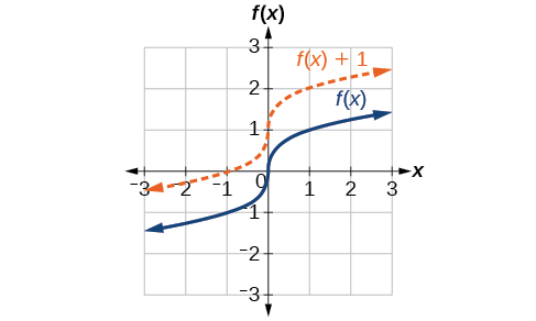
To help you visualize the concept of a vertical shift, consider that [latex],y=fleft(xright).,[/latex] Therefore,[latex],fleft(xright)+k,[/latex] is equivalent to [latex],y+k.,[/latex] Every unit of [latex],y,[/latex] is replaced by [latex],y+k,,[/latex] so the y-value increases or decreases depending on the value of [latex],k.,[/latex] The result is a shift upward or downward.
Vertical Shift
Given a function [latex]fleft(xright),[/latex] a new function [latex]gleft(xright)=fleft(xright)+k,[/latex] where [latex],k[/latex] is a constant, is a vertical shift of the function [latex]fleft(xright).[/latex] All the output values change by [latex]k[/latex] units. If [latex]k[/latex] is positive, the graph will shift up. If [latex]k[/latex] is negative, the graph will shift down.
Adding a Constant to a Function
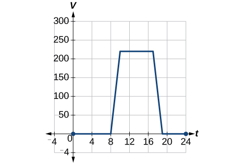
To regulate the temperature in a green building, airflow vents near the roof open and close throughout the day. Figure 3 shows the area of open vents [latex],V,[/latex] (in square feet) throughout the day in hours after midnight,[latex],t.,[/latex] During the summer, the facilities manager decides to try to better regulate temperature by increasing the amount of open vents by 20 square feet throughout the day and night. Sketch a graph of this new function.
Show Solution
We can sketch a graph of this new function by adding 20 to each of the output values of the original function. This will have the effect of shifting the graph vertically up, as shown in Figure 4.
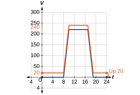
Notice that in Figure 4, for each input value, the output value has increased by 20, so if we call the new function[latex],Sleft(tright),[/latex] we could write
This notation tells us that for any value of[latex],t,Sleft(tright),[/latex] can be found by evaluating the function[latex],V,[/latex] at the same input and then adding 20 to the result. This defines[latex],S,[/latex]as a transformation of the function[latex],V,,[/latex] in this case, a vertical shift up 20 units. Notice that with a vertical shift, the input values stay the same and only the output values change. See Table 1.
| [latex]t[/latex] | 0 | 8 | 10 | 17 | 19 | 24 |
| [latex]V(t)[/latex] | 0 | 0 | 220 | 220 | 0 | 0 |
| [latex]S(t)[/latex] | 20 | 20 | 240 | 240 | 20 | 20 |
How To
Given a tabular function, create a new row to represent a vertical shift.
- Identify the output row or column.
- Determine the magnitude of the shift.
- Add the shift to the value in each output cell. Add a positive value for up or a negative value for down.
Shifting a Tabular Function Vertically
A function[latex],fleft(xright),[/latex]is given in Table 2. Create a table for the function[latex],gleft(xright)=fleft(xright)-3.[/latex]
| [latex]x[/latex] | 2 | 4 | 6 | 8 |
| [latex]f(x)[/latex] | 1 | 3 | 7 | 11 |
Show Solution
The formula[latex],gleft(xright)=fleft(xright)-3,[/latex] tells us that we can find the output values of [latex],g,[/latex] by subtracting 3 from the output values of[latex],f.,[/latex] For example:
Analysis
As with the earlier vertical shift, notice the input values stay the same and only the output values change.
Try It
The function[latex],hleft(tright)=-4.9{t}^{2}+30t,[/latex]gives the height[latex],h,[/latex]of a ball (in meters) thrown upward from the ground after[latex],t,[/latex]seconds. Suppose the ball was instead thrown from the top of a 10-m building. Relate this new height function[latex],bleft(tright),[/latex]to[latex],hleft(tright),,[/latex]and then find a formula for[latex],bleft(tright).[/latex]
Show Solution
Identifying Horizontal Shifts
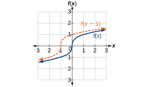
We just saw that the vertical shift is a change to the output, or outside, of the function. We will now look at how changes to input, on the inside of the function, change its graph and meaning. A shift to the input results in a movement of the graph of the function left or right in what is known as a horizontal shift, shown in Figure 5.
For example, if [latex],fleft(xright)={x}^{2},,[/latex] then [latex],gleft(xright)={left(x-2right)}^{2},[/latex] is a new function. Each input is reduced by 2 prior to squaring the function. The result is that the graph is shifted 2 units to the right, because we would need to increase the prior input by 2 units to yield the same output value as given in [latex],f.[/latex]
Horizontal Shift
Given a function [latex],f,,[/latex] a new function [latex],gleft(xright)=fleft(x-hright),,[/latex] where [latex],h,[/latex] is a constant, is a horizontal shift of the function [latex],f.,[/latex] If [latex],h,[/latex] is positive, the graph will shift right. If [latex],h,[/latex] is negative, the graph will shift left.
Adding a Constant to an Input
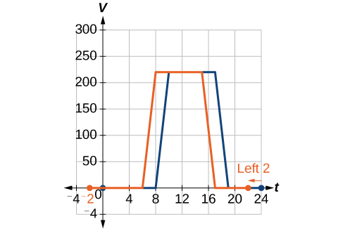
Returning to our building airflow example from Figure 3, suppose that in autumn, the facilities manager decides that the original venting plan starts too late and wants to begin the entire venting program 2 hours earlier. Sketch a graph of the new function.
Show Solution
We can set[latex],Vleft(tright),[/latex]to be the original program and [latex],Fleft(tright),[/latex] to be the revised program.
In the new graph, at each time, the airflow is the same as the original function [latex],V,[/latex] was 2 hours later. For example, in the original function [latex],V,,[/latex] the airflow starts to change at 8 a.m., whereas for the function[latex],F,,[/latex] the airflow starts to change at 6 a.m. The comparable function values are[latex],Vleft(8right)=Fleft(6right).,[/latex] See Figure 6. Notice also that the vents first opened to [latex],220{text{ ft}}^{2},[/latex] at 10 a.m. under the original plan, while under the new plan, the vents reach [latex],220{text{ ft}}^{text{2}},[/latex] at 8 a.m., so
[latex] V(10) = F(8)[/latex].
In both cases, we see that, because[latex],Fleft(tright),[/latex]starts 2 hours sooner,[latex],h=-2.,[/latex]That means that the same output values are reached when
[latex],Fleft(tright)=Vleft(t-left(-2right)right)=Vleft(t+2right).[/latex]
Analysis
Note that[latex],Vleft(t+2right),[/latex]has the effect of shifting the graph to the left.
Horizontal changes or “inside changes” affect the domain of a function (the input) instead of the range and often seem counterintuitive. The new function[latex],Fleft(tright),[/latex] uses the same outputs as[latex],Vleft(tright),,[/latex] but matches those outputs to inputs 2 hours earlier than those of[latex],Vleft(tright).,[/latex] Said another way, we must add 2 hours to the input of[latex],V,[/latex] to find the corresponding output for [latex]F: Fleft(tright)=Vleft(t+2right).[/latex]
How To
Given a tabular function, create a new row to represent a horizontal shift.
- Identify the input row or column.
- Determine the magnitude of the shift.
- Add the shift to the value in each input cell.
Shifting a Tabular Function Horizontally
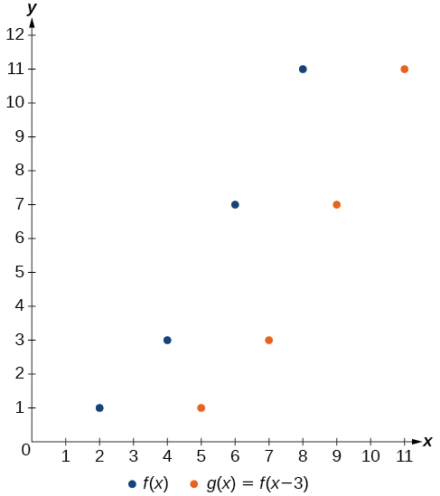
A function [latex],fleft(xright),[/latex] is given in Table 4. Create a table for the function[latex],gleft(xright)=fleft(x-3right).[/latex]
| [latex]x[/latex] | 2 | 4 | 6 | 8 |
| [latex]fleft(xright)[/latex] | 1 | 3 | 7 | 11 |
Show Solution
The formula[latex],gleft(xright)=fleft(x-3right),[/latex] tells us that the output values of[latex],g,[/latex] are the same as the output value of [latex],f,[/latex] when the input value is 3 less than the original value. For example, we know that [latex],fleft(2right)=1.,[/latex] To get the same output from the function[latex],g,,[/latex] we will need an input value that is 3 larger. We input a value that is 3 larger for [latex],gleft(xright),[/latex] because the function takes 3 away before evaluating the function [latex],f.[/latex]
We continue with the other values to create Table 5.
| [latex]x[/latex] | 5 | 7 | 9 | 11 |
| [latex]x-3[/latex] | 2 | 4 | 6 | 8 |
| [latex]fleft(x–3right)[/latex] | 1 | 3 | 7 | 11 |
| [latex]gleft(xright)[/latex] | 1 | 3 | 7 | 11 |
The result is that the function [latex],gleft(xright),[/latex] has been shifted to the right by 3. Notice the output values for [latex],gleft(xright),[/latex] remain the same as the output values for[latex],fleft(xright),,[/latex] but the corresponding input values, [latex],x,,[/latex] have shifted to the right by 3. Specifically, 2 shifted to 5, 4 shifted to 7, 6 shifted to 9, and 8 shifted to 11.
Analysis
Figure 7 represents both of the functions. We can see the horizontal shift in each point.
Identifying a Horizontal Shift of a Toolkit Function
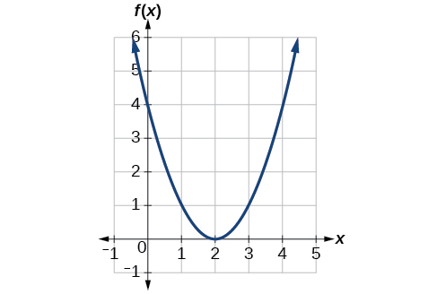
Figure 8 represents a transformation of the toolkit function [latex],fleft(xright)={x}^{2}.,[/latex] Relate this new function [latex],gleft(xright),[/latex]to[latex],fleft(xright),,[/latex] and then find a formula for[latex],gleft(xright).[/latex]
Show Solution
Notice that the graph is identical in shape to the [latex],fleft(xright)={x}^{2},[/latex] function, but the x-values are shifted to the right 2 units. The vertex used to be at (0,0), but now the vertex is at (2,0). The graph is the basic quadratic function shifted 2 units to the right, so
Notice how we must input the value [latex],x=2,[/latex] to get the output value [latex],y=0;,[/latex] the x-values must be 2 units larger because of the shift to the right by 2 units. We can then use the definition of the [latex],fleft(xright),[/latex] function to write a formula for [latex],gleft(xright),[/latex] by evaluating [latex],fleft(x-2right).[/latex]
Analysis
To determine whether the shift is [latex],+2,[/latex] or [latex],-2[/latex], consider a single reference point on the graph. For a quadratic, looking at the vertex point is convenient. In the original function,[latex],fleft(0right)=0.,[/latex] In our shifted function, [latex],gleft(2right)=0.,[/latex] To obtain the output value of 0 from the function[latex],f,,[/latex] we need to decide whether a plus or a minus sign will work to satisfy [latex],gleft(2right)=fleft(x-2right)=fleft(0right)=0.,[/latex] For this to work, we will need to subtract 2 units from our input values.
Interpreting Horizontal versus Vertical Shifts
The function [latex],Gleft(mright),[/latex] gives the number of gallons of gas required to drive [latex],m,[/latex] miles. Interpret [latex],Gleft(mright)+10,[/latex]and[latex],Gleft(m+10right).[/latex]
Show Solution
[latex]Gleft(mright)+10,[/latex] can be interpreted as adding 10 to the output, gallons. This is the gas required to drive[latex],m,[/latex] miles, plus another 10 gallons of gas. The graph would indicate a vertical shift.
[latex]Gleft(m+10right),[/latex] can be interpreted as adding 10 to the input, miles. So this is the number of gallons of gas required to drive 10 miles more than [latex],m,[/latex] miles. The graph would indicate a horizontal shift.
Try It
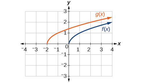
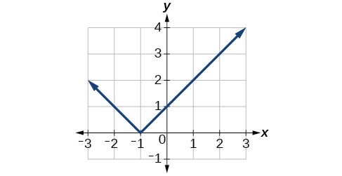
Given the function [latex],fleft(xright)=sqrt{x},,[/latex] graph the original function [latex],fleft(xright),[/latex] and the transformation [latex],gleft(xright)=fleft(x+2right),[/latex] on the same axes. Is this a horizontal or a vertical shift? Which way is the graph shifted and by how many units?
Show Solution
The graphs of [latex],fleft(xright),[/latex] and [latex],gleft(xright),[/latex] are shown below. The transformation is a horizontal shift. The function is shifted to the left by 2 units.
Combining Vertical and Horizontal Shifts
Now that we have two transformations, we can combine them. Vertical shifts are outside changes that affect the output (y-) values and shift the function up or down. Horizontal shifts are inside changes that affect the input (x-) values and shift the function left or right. Combining the two types of shifts will cause the graph of a function to shift up or down and left or right.
How To
Given a function and both a vertical and a horizontal shift, sketch the graph.
- Identify the vertical and horizontal shifts from the formula.
- The vertical shift results from a constant added to the output. Move the graph up for a positive constant and down for a negative constant.
- The horizontal shift results from a constant added to the input. Move the graph left for a positive constant and right for a negative constant.
- Apply the shifts to the graph in either order.
Graphing Combined Vertical and Horizontal Shifts
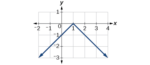
Given [latex],fleft(xright)=|x|,,[/latex] sketch a graph of [latex],hleft(xright)=fleft(x+1right)-3.[/latex]
Show Solution
The function [latex],f,[/latex] is our toolkit absolute value function. We know that this graph has a V shape, with the point at the origin. The graph of [latex],h,[/latex] has transformed [latex],f,[/latex] in two ways: [latex],fleft(x+1right),[/latex] is a change on the inside of the function, giving a horizontal shift left by 1, and the subtraction by 3 in [latex],fleft(x+1right)-3,[/latex] is a change to the outside of the function, giving a vertical shift down by 3. The transformation of the graph is illustrated in Figure 9.
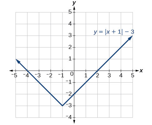
Let us follow one point of the graph of [latex],fleft(xright)=|x|.[/latex]
- The point [latex]left(0,0right)[/latex] is transformed first by shifting left 1 unit:[latex]left(0,0right)to left(-1,0right)[/latex]
- The point[latex]left(-1,0right)[/latex] is transformed next by shifting down 3 units:[latex]left(-1,0right)to left(-1,-3right)[/latex]
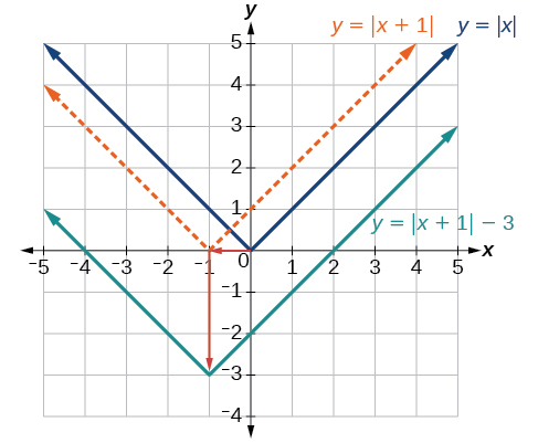
Figure 10 shows the graph of [latex],h.[/latex]
Try It
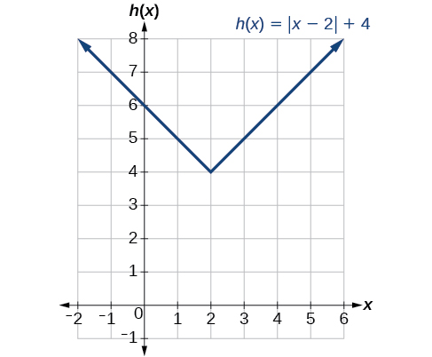
Given [latex],fleft(xright)=|x|,,[/latex] sketch a graph of [latex],hleft(xright)=fleft(x-2right)+4.[/latex]
Show Solution
Identifying Combined Vertical and Horizontal Shifts
Write a formula for the graph shown in Figure 11, which is a transformation of the toolkit square root function.
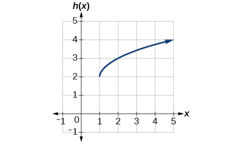
Show Solution
The graph of the toolkit function starts at the origin, so this graph has been shifted 1 to the right and up 2. In function notation, we could write that as
Using the formula for the square root function, we can write
Analysis
Note that this transformation has changed the domain and range of the function. This new graph has domain [latex],left[1,infty right),[/latex] and range [latex],left[2,infty right).[/latex]
Try It
Write a formula for a transformation of the toolkit reciprocal function [latex],fleft(xright)=frac{1}{x},[/latex] that shifts the function’s graph one unit to the right and one unit up.
Show Solution
[latex]gleft(xright)=frac{1}{x-1}+1[/latex]
Graphing Functions Using Reflections about the Axes
Another transformation that can be applied to a function is a reflection over the x– or y-axis. A vertical reflection reflects a graph vertically across the x-axis, while a horizontal reflection reflects a graph horizontally across the y-axis. The reflections are shown in Figure 12.
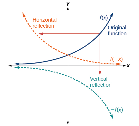
Notice that the vertical reflection produces a new graph that is a mirror image of the base or original graph about the x-axis. The horizontal reflection produces a new graph that is a mirror image of the base or original graph about the y-axis.
Reflections
Given a function [latex],fleft(xright),[/latex] a new function [latex],gleft(xright)=-fleft(xright),[/latex] is a vertical reflection of the function [latex],fleft(xright),,[/latex] sometimes called a reflection about (or over, or through) the x-axis.
Given a function [latex],fleft(xright),,[/latex] a new function [latex],gleft(xright)=fleft(-xright),[/latex] is a horizontal reflection of the function [latex],fleft(xright),,[/latex] sometimes called a reflection about the y-axis.
How To
Given a function, reflect the graph both vertically and horizontally.
- Multiply all outputs by –1 for a vertical reflection. The new graph is a reflection of the original graph about the x-axis.
- Multiply all inputs by –1 for a horizontal reflection. The new graph is a reflection of the original graph about the y-axis.
Reflecting a Graph Horizontally and Vertically
Reflect the graph of [latex],sleft(tright)=sqrt{t}[/latex] (a) vertically and (b) horizontally.
Show Solution
- Reflecting the graph vertically means that each output value will be reflected over the horizontal t-axis, as shown in Figure 13.
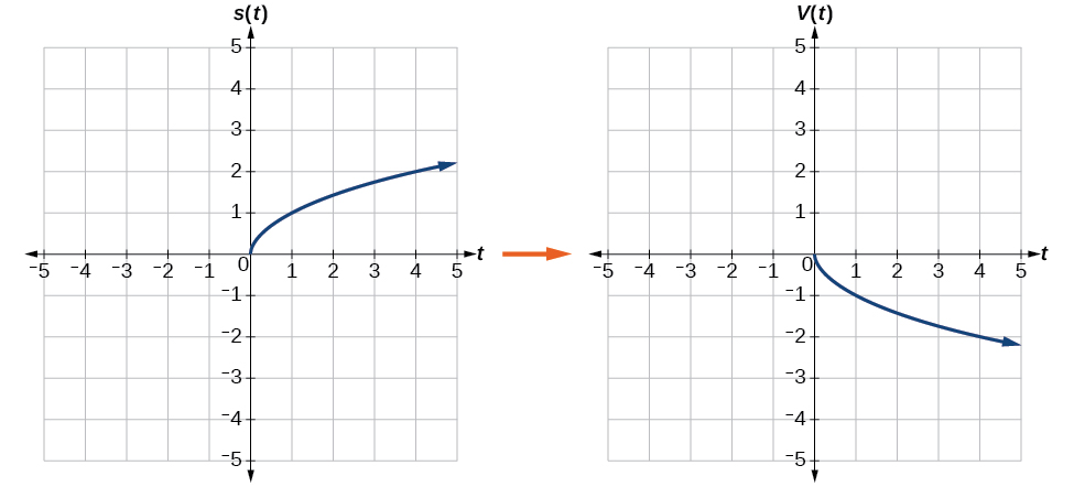
Figure 13. Vertical reflection of the square root function Because each output value is the opposite of the original output value, we can write
[latex]Vleft(tright)=-sleft(tright)text{ or }Vleft(tright)=-sqrt{t}[/latex]Notice that this is an outside change, or vertical shift, that affects the output [latex],sleft(tright),[/latex] values, so the negative sign belongs outside of the function.
- Reflecting horizontally means that each input value will be reflected over the vertical axis, as shown in Figure 14.
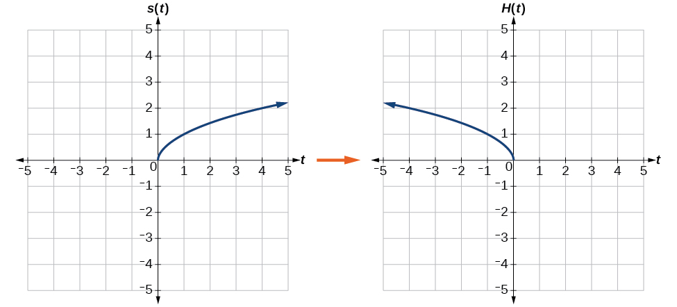
Figure 14. Horizontal reflection of the square root function Because each input value is the opposite of the original input value, we can write
[latex]Hleft(tright)=sleft(-tright)text{ or }Hleft(tright)=sqrt{-t}[/latex]Notice that this is an inside change or horizontal change that affects the input values, so the negative sign is on the inside of the function.
Note that these transformations can affect the domain and range of the functions. While the original square root function has domain [latex],left[0,infty right),[/latex] and range [latex],left[0,infty right),,[/latex] the vertical reflection gives the [latex],Vleft(tright),[/latex] function the range [latex]left(-infty ,,0right][/latex] and the horizontal reflection gives the[latex],Hleft(tright),[/latex] function the domain [latex]left(-infty ,,0right].[/latex]
Try It
Reflect the graph of [latex],fleft(xright)=|x-1|[/latex] (a) vertically and (b) horizontally.
Show Solution
Reflecting a Tabular Function Horizontally and Vertically
A function[latex],fleft(xright),[/latex] is given as Table 6. Create a table for the functions below.
- [latex],gleft(xright)=-fleft(xright)[/latex]
- [latex],hleft(xright)=fleft(-xright)[/latex]
| [latex]x[/latex] | 2 | 4 | 6 | 8 |
| [latex]fleft(xright)[/latex] | 1 | 3 | 7 | 11 |
Show Solution
- For [latex],gleft(xright),,[/latex] the negative sign outside the function indicates a vertical reflection, so the x-values stay the same and each output value will be the opposite of the original output value. See Table 7.
Table 7 [latex]x[/latex] 2 4 6 8 [latex],gleft(xright),[/latex] –1 –3 –7 –11 - For [latex],hleft(xright),,[/latex] the negative sign inside the function indicates a horizontal reflection, so each input value will be the opposite of the original input value and the [latex],hleft(xright),[/latex] values stay the same as the [latex],fleft(xright),[/latex] values. See Table 8.
Table 8 [latex]x[/latex] −2 −4 −6 −8 [latex]hleft(xright)[/latex] 1 3 7 11
Try It
A function [latex],fleft(xright),[/latex] is given as Table 9. Create a table for the functions below.
- [latex]gleft(xright)=-fleft(xright)[/latex]
- [latex]hleft(xright)=fleft(-xright)[/latex]
| [latex]x[/latex] | −2 | 0 | 2 | 4 |
| [latex]fleft(xright)[/latex] | 5 | 10 | 15 | 20 |
Show Solution
- [latex]gleft(xright)=-fleft(xright)[/latex]
[latex]x[/latex] -2 0 2 4 [latex]gleft(xright)[/latex] [latex]-5[/latex] [latex]-10[/latex] [latex]-15[/latex] [latex]-20[/latex] - [latex]hleft(xright)=fleft(text{−}xright)[/latex]
[latex]x[/latex] 2 0 -2 -4 [latex]hleft(xright)[/latex] [latex]5[/latex] [latex]10[/latex] [latex]15[/latex] [latex]20[/latex]
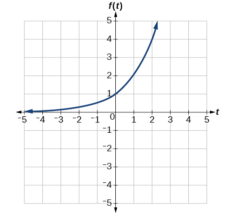
Applying a Learning Model Equation
A common model for learning has an equation similar to [latex]kleft(tright)=-{2}^{-t}+1,,[/latex] where [latex]k[/latex] is the percentage of mastery that can be achieved after [latex]t[/latex] practice sessions. This is a transformation of the function [latex]fleft(tright)={2}^{t}[/latex], shown in Figure 15. Sketch a graph of [latex]kleft(tright).[/latex]
Show Solution
This equation combines three transformations into one equation.
- A horizontal reflection:[latex]fleft(text{−}tright)={2}^{-t}[/latex]
- A vertical reflection:[latex],-fleft(text{−}tright)=-{2}^{-t}[/latex]
- A vertical shift:[latex],-fleft(text{−}tright)+1=-{2}^{-t}+1[/latex]
We can sketch a graph by applying these transformations one at a time to the original function. Let us follow two points through each of the three transformations. We will choose the points (0, 1) and (1, 2).
- First, we apply a horizontal reflection: (0, 1) (–1, 2).
- Then, we apply a vertical reflection: (0, -1) (-1, –2)
- Finally, we apply a vertical shift: (0, 0) (-1, -1)).
This means that the original points, (0,1) and (1,2), become (0,0) and (-1,-1) after we apply the transformations.
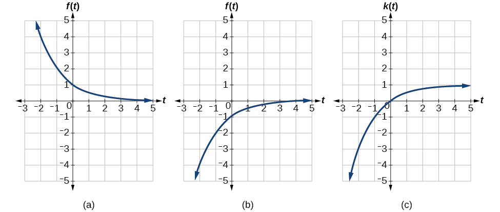
In Figure 16, the first graph results from a horizontal reflection. The second results from a vertical reflection. The third results from a vertical shift up 1 unit.
Analysis
As a model for learning, this function would be limited to a domain of [latex],tge 0,,[/latex] with corresponding range [latex],left[0,1right).[/latex]
Media Attributions
- 3.6 Figure 2 © OpenStax Algebra and Trigonometry, 2e is licensed under a CC BY (Attribution) license
- 3.6 Figure 3 © OpenStax Algebra and Trigonometry, 2e is licensed under a CC BY (Attribution) license
- 3.6 Figure 4 © OpenStax Algebra and Trigonometry, 2e is licensed under a CC BY (Attribution) license
- 3.6 Figure 5 © OpenStax Algebra and Trigonometry, 2e is licensed under a CC BY (Attribution) license
- 3.6 Figure 6 © OpenStax Algebra and Trigonometry, 2e is licensed under a CC BY (Attribution) license
- 3.6 Figure 7 © OpenStax Algebra and Trigonometry, 2e is licensed under a CC BY (Attribution) license
- 3.6 Figure 8 © OpenStax Algebra and Trigonometry, 2e is licensed under a CC BY (Attribution) license
- 3.6 Figure 9 © OpenStax Algebra and Trigonometry, 2e is licensed under a CC BY (Attribution) license
- 3.6 Figure 10 © OpenStax Algebra and Trigonometry, 2e is licensed under a CC BY (Attribution) license
- 3.6 Figure 11 © OpenStax Algebra and Trigonometry, 2e is licensed under a CC BY (Attribution) license
- 3.6 Figure 12 © OpenStax Algebra and Trigonometry, 2e is licensed under a CC BY (Attribution) license
- 3.6 Figure 13 © OpenStax Algebra and Trigonometry, 2e is licensed under a CC BY (Attribution) license
- 3.6 Figure 14 © OpenStax Algebra and Trigonometry, 2e is licensed under a CC BY (Attribution) license
- 3.6 Figure 15 © OpenStax Algebra and Trigonometry, 2e is licensed under a CC BY (Attribution) license
- 3.6 Figure 16 © OpenStax Algebra and Trigonometry, 2e is licensed under a CC BY (Attribution) license
