Spreadsheets

 

LEARN IT

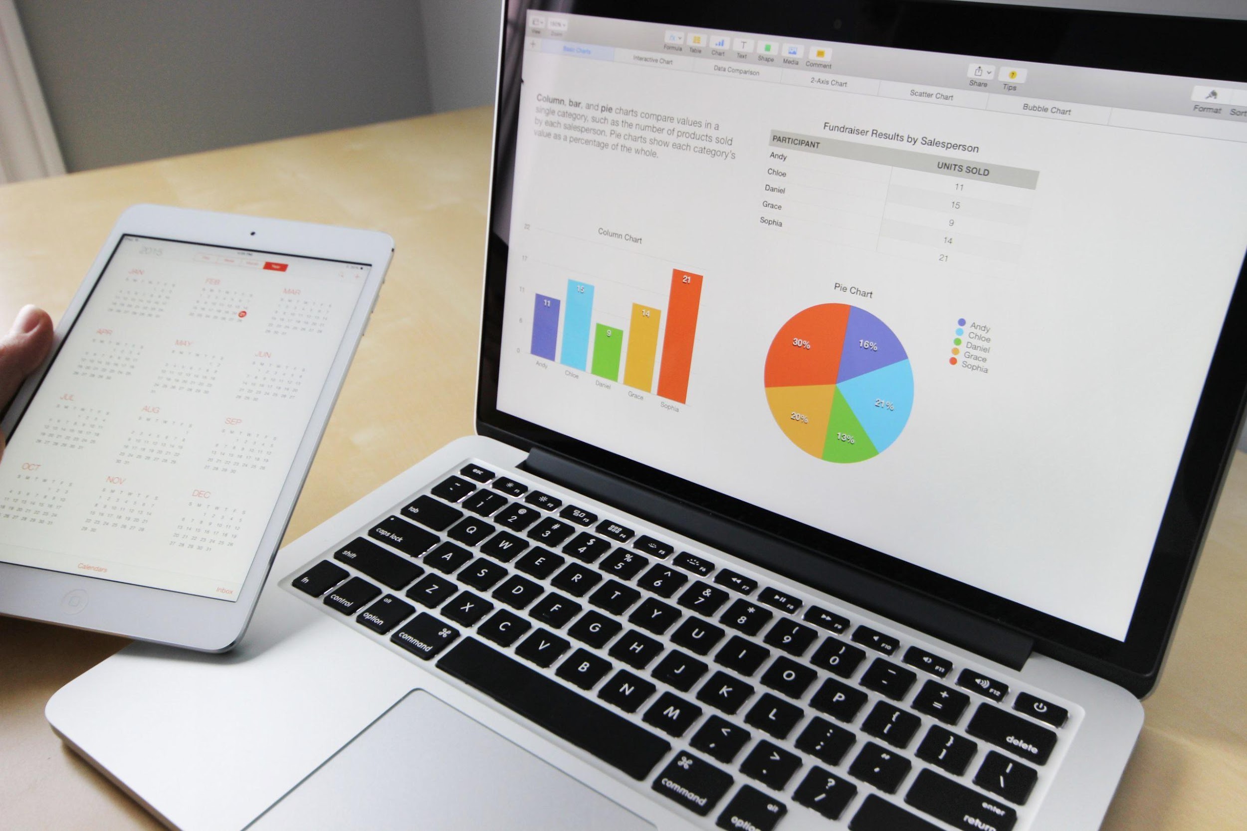
A spreadsheet is a file with cells in rows and columns. A spreadsheet helps arrange, calculate, and sort data. Data in a spreadsheet can be numeric values, text, formulas, references, and functions. We will even learn how to embed charts and graphs into a spreadsheet. Spreadsheets are used to visualize data in a meaningful way that can be used to make complex decisions. Spreadsheets are the most basic tool in data science. Spreadsheets can take raw data, and tell a story with it.

Common Spreadsheet Software:

Software Name	Type	Key Features
Microsoft Excel	Commercial	Runs on Windows and MacPart of Office 365. Recent features include robust formulas and functions, charts, graphs, and sparklines. Arguably the most popular spreadsheet software.
Google Sheets	Online—Part of the free, web-based Google Docs Editors suite	Allows users to create, view, and edit spreadsheets online while collaborating with other users in real-time. Available as a web application supported on most web browsers. Compatible with Google Drive.
LibreOffice Calc	Free and open-source office productivity software suite	Uses the OpenDocument standard, but supports formats of most other major office suites, including Microsoft Office. Official support for Microsoft Windows, macOS, and Linux. It has several unique features, including a system that automatically defines a series of graphs, based on information available to the user.
Apple Numbers	Online—Part of the iWork productivity suite	Runs on the MacOS, iPadOS, and iOS operating systems.

Going forward, we will focus on Microsoft Excel and LibreOffice Calc.

SPREADSHEET PRACTICE 1

There are many similarities across spreadsheet software, so the skills we are learning can be translated to any other software and apps. The following assignments are designed to be completed using either Microsoft Excel in Office 365 or LibreOffice Calc on a PC with Windows 10 or higher.

We will use spreadsheet software to perform Data Analysis including complex calculations, analyze data so that we can make intelligent decisions, and create visually interesting charts and graphs that help us understand the data. It is best to use a keyboard and mouse or touchpad rather than a touchscreen when working with spreadsheets.

In a spreadsheet, data is stored in a cell. Cell content is anything that is stored in the cell and can be either a constant value or a formula. The most used values are text values and number values. Values can also be a date or time. A text value is also referred to as a label.

Prefer to watch and learn? Check out this video tutorial:

 

Complete the following Practice Activity and submit your completed project.

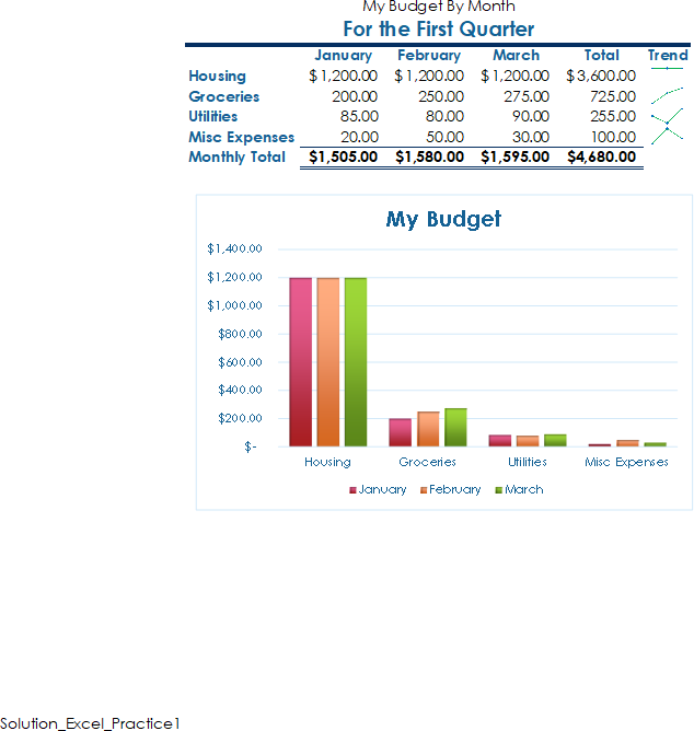
For our first assignment, we will create a spreadsheet with monthly expenses. We will go over the activity with both software: Microsoft Excel and LibreOffice Calc. When the instructions for both spreadsheet applications are different, the Microsoft Excel steps will be shown at the left, and the LibreOffice Calc steps at the right. However, most of the instructions are identical.

• We will start with a new blank spreadsheet.

Start Excel. Click Blank Workbook.

Start LibreOffice Calc.

• Select File, Save As, Browse, and then navigate to your folder on your flash drive or other location where you save your files. Name the file depending on the software you are using as

Yourlastname_Yourfirstname_Excel_Practice_1, if you are using Microsoft Excel.

Yourlastname_Yourfirstname_Calc_Practice_1, if you are using LibreOffice Calc.

• Take a moment to locate the following components of the spreadsheet window. Notice how Columns are lettered and Rows are numbered. The intersection of a row and column is a cell. The active cell in the image is A1.
  • Microsoft Excel

• • LibreOffice Calc

• Notice the vertical and horizontal scroll bars. Use the arrows to practice scrolling on the page.
• In cell A1, type My Budget By Month and press Enter.
• In cell A2 Type For the First Quarter and press Enter.
• In the Name Box, change A3 to A4 and then Hit Enter. Notice how the active cell changed to A4. The Name Box is the little window just above the spreadsheet in the left corner.
• Starting in cell A4, Type each of the following, pressing Enter after each:
  • Housing
  • Groceries
  • Utilities
  • Misc. Expenses
  • Monthly Total
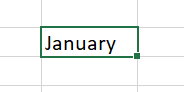
• In cell B3, type January and press Enter.
• Select cell B3 and use the fill handle to drag to cell D3. Notice how the names of the months automatically generate. The fill handle enables autofill, which generates and extends a series of values into adjacent cells based on the value of other cells.

• Adjust the column width for column A by dragging the right boundary until all the text is displayed in the cells.
• Select the range B3:D3 and center the text.

On the Home Tab, Paragraph Group, choose Center.

On the Formatting Toolbar, choose Align Center

• In cell B4, type 1200 and enter the remaining numbers as shown:

	January	February	March
Housing	1200	1200	1200
Groceries	200	250	275
Utilities	85	80	90
Misc Expenses	20	50	30

• In cell B8, type =b4 + b5 + b6 + b7 and press Tab.
• In cell C8, type =c4 + c5 + c6 + c7 and press Tab.

Note: Using this technique we are manually entering a formula that sums a range of cells. Notice the Formula Bar as you enter your formula. The formula bar displays the Underlying Formula.

• A quicker way to enter a formula is with a function. We will use the SUM function next. In cell D8, type =SUM(D4:D7) and press Enter. You can also type =SUM( and select the range of cells D4 to D7.
• In cell E3, type Total and then press Enter.
• Click in cell E4; Press Alt + =. This is a keyboard shortcut that enters the Sum function. If the keyboard shortcut does not work (this is common due to variations in keyboards), use the technique for using the SUM function described previously.
• With Cell E4 selected, drag the fill handle in cell E4 down through cell E8.
• Click in cell F3, type Trend, and press Enter.
• Click in cell A1 and drag your cursor to the right to select the range A1:F1.

On the Home tab, in the Alignment Group, choose Merge and Center.

On the Format Tab, Merge Cells, choose Merge and Center Cells.

• The title should be Merged and centered in the range A1:F1.
• Using the same technique, merge and center the title in the range A2:F2.

Apply the Title style to cell A1 and the Heading 1 style to cell A2. Cell styles are on the Home Tab, Styles Group, then choose the arrow next to cell styles.

Apply the Heading 1 style to cell A1 and the Heading 2 style to cell A2. Cell styles are on the Styles Tab of the Menu bar.

Apply the Heading 4 style to the ranges B3:F3 and A4:A8.

Apply the Accent 3 style (under the Styles Tab) to the ranges B3:F3 and A4:A8.

• You can select the first range, hold down the CTRL key, and select the second range, then apply the cell style. Or apply, one at a time.

Apply the Accounting number format to the ranges B4:E4 and B8:E8. The number format is located on the Home Tab, Number Group. Select the arrow to view a drop-down list of all number formats

Apply the Currency Format under the Formatting Toolbar, and choose the Default.

Apply the Comma number style to the range B5:E7. This is located on the Home Tab, Number Group. Select the comma.

Apply the Format as Number located on the Formatting Toolbar to the range B5:E7.

Apply the Total number style to the range B8:E8. Cell styles are on the Home Tab, Styles Group. Then choose the arrow next to cell styles.

To the range B8:E8, first apply Bold lettering, then apply Borders and choose top and bottom borders. Both are in the Formatting Toolbar.

• AutoFit column D. Select column D by clicking on the D Column Header. Then, double-click the line between the D and E.

Or, with Column D selected, on the Home Tab, Cells Group, click the arrow next to Format and choose Autofit for the Column.

Or, with Column D selected, on the Menu Bar, choose Format tab, Columns, and Optimal Fit.

Apply the Slice theme to the Workbook. On the Page Layout Tab, in the Themes Group, choose Slice. If necessary, adjust the total cells, or any other cells to ensure you can see all of the cell content.

• Select the range A3:D7.

With the chart selected, under Chart Tools, in the Chart Design Tab, in the Chart Layouts Group, choose the Add Chart Element and ensure the Chart Title is Above Chart. Change the Chart Title to My Budget.

With the chart selected, under Insert, choose Titles. Then, change the Chart Title to My Budget.

On the Insert tab, in the charts group, click Recommended Charts, click All Charts, and select Cluster Column chart.

On the Insert tab, in the Chart group, click Column chart, the leftmost option.

 

Using Change Colors select Colorful 4. Change colors located on the Chart Tools, Design Tab, under Chart Styles.

To change the chart colors and transparency, double-click each of the columns to open a window menu, and choose Color, the required Palette, and the specific color. Then, in Transparency, choose Gradient, Linear, and one Start value and one End value.

• Drag the chart by clicking and holding any of the chart’s outer lines. Move the chart so that the upper left corner is inside cell A10.

Ensure the chart is still selected, and apply Chart styles, Style 6. Chart styles are located on the Chart Tools, Design Tab, under Chart Styles. Click the down arrow to see all the Chart Styles.

You can customize all the elements of your chart separately

• Select the range B4:D4 and insert a Line sparkline in cell F4. Be sure to not include the totals in the sparkline range.
• Sparklines are located on the Insert Tab. In the Sparklines group, choose Line. The sparkline will display in cell F4. For the location range, click into cell F4.

With cell F4 selected, on the Sparklines, Design Toolbar, in the Show group choose the checkbox next to Markers.

Apply the Sparkline Style Colorful #4 style. Styles are located on the Sparkline Design toolbar in the Style group. Choose the down arrow to view more styles.

With cell F4 selected, use the fill handle to fill the sparkline to cells F5:F7.

On the Page Layout Tab, Sheet Options Group, click the arrow to launch the Page Setup Dialog Box. Notice how it opens to the Sheet tab. Go to the Margins tab and click the checkbox to center the data and chart horizontally on the page.

On the Menu Bar, Format, click Page Style. Go to Page, Layout Settings, and choose Horizontal Table alignment. Click OK.

Open the Page Setup Dialog Box, go to the Header/Footer tab. Choose Custom Footer and insert the File Name in the left section of the footer.

On the Menu Bar, Format, click Page Style. Choose Footer, and click Footer on. Then, click Edit. And chose the File Name followed by the page number between the options displayed.

• The file name will show in the Print Preview and also when the spreadsheet is printed. This is a field, so if the file name is changed, it will automatically update the footer with the new file name.

Click File to go to Backstage View. Under Info, choose Properties, and then Advanced Properties. Add the following Properties: Title: Excel Budget Subject: Course name and Section # Author: Your First and Last Name Keywords: Sums, Charts, Budget, Excel

Click Tools, Options under LibreOffice File to go to Backstage View. Under Info, choose Properties, and then Advanced Properties. Add the following Properties: Title: LibreOffice Budget Subject: Course name and Section # Author: Your First and Last Name Keywords: Sums, Charts, Budget, LibreOffice

 

• Click the back arrow to exit Backstage view. Click the Save shortcut button and ensure your file is saved in a safe location.
• Select the range A2:F5 and then press Ctrl + F2. This is the keyboard shortcut that displays Print Preview. If you do not have the shortcut key, click File to enter Backstage View, Print, and view the Print Preview.
• Change the print settings option to Print Selection and notice how the Print Preview changes. Printing of this assignment is not required, but if you needed to print a copy, you would click Print.
• Exit Backstage view and Save your file.
• On the Formulas tab, in the Formulas Auditing group, Show the Formulas. This is a toggle button, so press it once to show the formulas. Press it again to hide the formulas. Notice how row 8 displays the formula rather than the result when Show the Formulas is turned on.
• On the Page Layout tab, in the Page Setup group, Change to Landscape orientation and Scale the data to fit on one page. This is on the Page Tab of the Page Layout Dialog Box.
• Run spelling and grammar check, compare your file to the image below, and make all necessary corrections.
• Submit as instructed by your instructor.