Describe the effect of parameters in polar curves.
Compare polar and Cartesian graphs.
Sketch standard polar graphs.
Identify standard polar graphs.
Write equations for standard polar graphs.
Find intersection points of polar graphs.
Graphing in Polar Coordinates
When we plot points in Cartesian coordinates, we start at the origin and move a distance right or left given by the [latex]x[/latex]-coordinate of the point, then move up or down according to the [latex]y[/latex]-coordinate. When we sketch the graph of an equation or function, we think of drawing the graph from left to right, with the "height" of the graph at each [latex]x[/latex]-value given by the function, as shown in figure (a).
In polar coordinates, however, the dependent variable, [latex]r\text{,}[/latex] gives not a height but a distance from the pole in direction [latex]\theta\text{,}[/latex] as shown in figure (b). When graphing an equation in polar coordinates, we think of sweeping around the pole in the counterclockwise direction, and at each angle [latex]\theta[/latex] the [latex]r[/latex]-value tells us how far the graph is from the pole.
Example 10.17.
Graph the polar equation [latex]r=2\sin \theta\text{.}[/latex]
Solution
We make a table of values, choosing the special values for [latex]\theta\text{.}[/latex] For each value of [latex]\theta\text{,}[/latex] we evaluate [latex]r=2\sin \theta\text{.}[/latex]
[latex]\theta[/latex]
[latex]0[/latex]
[latex]\dfrac{\pi}{6}[/latex]
[latex]\dfrac{\pi}{4}[/latex]
[latex]\dfrac{\pi}{3}[/latex]
[latex]\dfrac{\pi}{2}[/latex]
[latex]\dfrac{2\pi}{3}[/latex]
[latex]\dfrac{3\pi}{4}[/latex]
[latex]\dfrac{5\pi}{6}[/latex]
[latex]\pi[/latex]
[latex]r[/latex]
[latex]0[/latex]
[latex]1[/latex]
[latex]\sqrt{2}[/latex]
[latex]\sqrt{3}[/latex]
[latex]2[/latex]
[latex]\sqrt{3}[/latex]
[latex]\sqrt{2}[/latex]
[latex]1[/latex]
[latex]0[/latex]
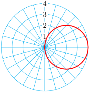
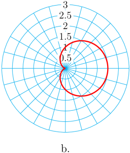
First we'll plot the points in the first quadrant. Observe that as [latex]\theta[/latex] increases from [latex]0[/latex] to [latex]\dfrac{\pi}{2}\text{,}[/latex] [latex]r[/latex] increases from [latex]0[/latex] to [latex]2\text{.}[/latex] Starting at the pole, we connect the points in order of increasing [latex]\theta\text{.}[/latex] Imagine a radial line sweeping around the graph through the first quadrant: as the angle increases, the length of the segment increases so that its tip traces out the graph shown in figure (a).
Now continue plotting the points in the table as [latex]\theta[/latex] increases from [latex]\dfrac{\pi}{2}[/latex] to [latex]\pi\text{.}[/latex] In the second quadrant, [latex]r[/latex] decreases as [latex]\theta[/latex] increases, as shown in figure (b). The graph we obtain is, in fact, a circle, which we will prove algebraically shortly. However, we have not yet plotted points for [latex]\theta[/latex] between [latex]0[/latex] and [latex]2\pi\text{.}[/latex] Because [latex]\sin \theta[/latex] is negative in the third and fourth quadrants, all the [latex]r[/latex]-values for these angles are negative.
[latex]\theta[/latex]
[latex]\pi[/latex]
[latex]\dfrac{7\pi}{6}[/latex]
[latex]\dfrac{5\pi}{4}[/latex]
[latex]\dfrac{4\pi}{3}[/latex]
[latex]\dfrac{3\pi}{2}[/latex]
[latex]\dfrac{5\pi}{3}[/latex]
[latex]\dfrac{7\pi}{4}[/latex]
[latex]\dfrac{11\pi}{6}[/latex]
[latex]\pi[/latex]
[latex]r[/latex]
[latex]0[/latex]
[latex]-1[/latex]
[latex]-\sqrt{2}[/latex]
[latex]-\sqrt{3}[/latex]
[latex]-2[/latex]
[latex]-\sqrt{3}[/latex]
[latex]-\sqrt{2}[/latex]
[latex]-1[/latex]
[latex]0[/latex]
When we plot the points in this table, we see that the original graph is traced out again. For example, the point [latex]\left(\dfrac{7\pi}{6}, -1\right)[/latex] is the same as the point [latex]\left(\dfrac{\pi}{6}, 1\right)\text{,}[/latex] the point [latex]\left(\dfrac{5\pi}{4}, -\sqrt{2}\right)[/latex] is the same as the point [latex]\left(\dfrac{\pi}{4}, \sqrt{2}\right)\text{,}[/latex] and so on, around the circle. Thus, the graph of [latex]r=2\sin \theta[/latex] is a circle, traced twice for [latex]0 \le \theta \le 2\pi\text{.}[/latex]
To prove that the graph in Example 1 is really a circle, we convert the equation [latex]r=2\sin \theta[/latex] to Cartesian form. First, multiply both sides by [latex]r[/latex] to obtain
[latex]r^2=2r\sin \theta[/latex]
Next, replace [latex]r^2[/latex] by [latex]x^2+y^2[/latex] and [latex]r\sin \theta[/latex] by [latex]y\text{,}[/latex] to get
[latex]x^2+y^2 = 2y[/latex]
This equation is quadratic in two variables, so its graph is a conic section. We put the equation in standard form by completing the square in [latex]y\text{.}[/latex]
[latex]x^2+y^2 - 2y = 0[/latex]
[latex]x^2+(y^2-2y {+1}) ={1} ~~~~~~~ \text{Add 1 to both sides.}[/latex]
[latex](x-0)^2 + (y-1)^2 = 1 ~~~~ \text{Write the equation in standard form.}[/latex]
We have the equation of a circle with center [latex](0,1)[/latex] and radius [latex]1\text{.}[/latex]
Checkpoint 10.18.
Graph the polar equation [latex]r=4\cos\theta\text{.}[/latex]
Solution
Using a Graphing Calculator
You are familiar with the graphs of many equations in Cartesian coordinates, including lines, parabolas and other conic sections, and the graphs of basic functions. You should now become familiar with some standard graphs in polar coordinates. These include circles and roses, cardioids and limaçons, lemniscates, and spirals.
At the end of this section, you will find a Catalog of the basic polar graphs and their properties. You can use your calculator, set in Polar mode, to experiment with these graphs.
Example 10.19.
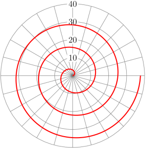
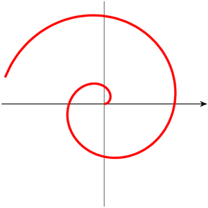
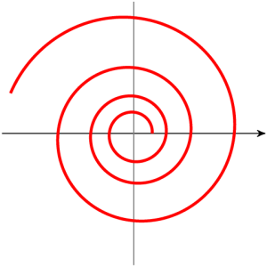
Graph the Archimedean spiral [latex]r=2\theta\text{,}[/latex] for [latex]0 \le \theta \le 6\pi\text{.}[/latex]
Solution
After setting the calculator in Polar mode, we enter the equation [latex]r=2\theta[/latex] and enter the window settings
We then press Zoom 5 to set a square window. The graph is shown at right.
Studying a table of values can help us understand the shape of the graph.
[latex]\theta[/latex]
[latex]0.25[/latex]
[latex]0.50[/latex]
[latex]0.75[/latex]
[latex]1.00[/latex]
[latex]1.25[/latex]
[latex]r[/latex]
[latex]0.50[/latex]
[latex]1.00[/latex]
[latex]1.50[/latex]
[latex]2.00[/latex]
[latex]2.50[/latex]
As [latex]\theta[/latex] increases, [latex]r[/latex] increases also, at a constant rate. We wind our way around the pole, steadily increasing our distance from the pole as we go. We spiral outward, tracing the graph shown above.
Checkpoint 10.20.
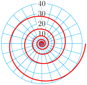
Use a calculator to graph the polar equation [latex]r=e^{0.1\theta}\text{.}[/latex] Use the window settings[latex]\theta\text{ min}=0~~~~~~~~~~\theta\text{ max}=12\pi~~~~~\theta\text{ step}=0.5[/latex]
[latex]\text{Xmin}=-45~~~~\text{Xmax}=45~~~~~~\text{Xstep}=10[/latex]
[latex]\text{Ymin}=-35~~~~\text{Ymax}=35~~~~~~~~~~\text{Yscl}=10[/latex]
Solution
It is important to connect the points on the graph in order of increasing [latex]\theta\text{.}[/latex]
Example 10.21.
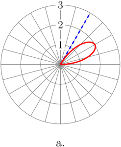
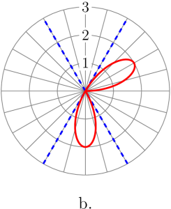
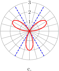
Graph the polar equation [latex]r=2\sin 3\theta\text{.}[/latex]
Solution
We'll graph the equation in stages in order to see how the graph is traced out. Begin with the window settings
Watch as your calculator produces the graph shown in figure (a).
Observe that as [latex]\theta[/latex] increases from [latex]0[/latex] to [latex]\dfrac{\pi}{3}\text{,}[/latex] [latex]r[/latex] first increases, reaching its maximum value of 2 at [latex]\theta = \dfrac{\pi}{6}[/latex] and then decreases back to 0. You can verify the values in the table below, which shows the points at multiples of [latex]\dfrac{\pi}{18}\text{.}[/latex] These points create the first loop of the graph.
[latex]\theta[/latex]
[latex]0[/latex]
[latex]\dfrac{\pi}{18}[/latex]
[latex]\dfrac{\pi}{9}[/latex]
[latex]\dfrac{\pi}{6}[/latex]
[latex]\dfrac{2\pi}{9}[/latex]
[latex]\dfrac{5\pi}{18}[/latex]
[latex]\dfrac{\pi}{3}[/latex]
[latex]3\theta[/latex]
[latex]0[/latex]
[latex]\dfrac{\pi}{6}[/latex]
[latex]\dfrac{\pi}{3}[/latex]
[latex]\dfrac{\pi}{2}[/latex]
[latex]\dfrac{2\pi}{3}[/latex]
[latex]\dfrac{5\pi}{6}[/latex]
[latex]\pi[/latex]
[latex]r[/latex]
[latex]0[/latex]
[latex]1[/latex]
[latex]\sqrt{3}[/latex]
[latex]2[/latex]
[latex]\sqrt{3}[/latex]
[latex]1[/latex]
[latex]0[/latex]
Next, change [latex]\theta\text{ max}[/latex] to [latex]\dfrac{2\pi}{3}\text{,}[/latex] and graph again. This time the calculator traces out two loops, as shown in figure (b). For [latex]\theta[/latex] between [latex]\dfrac{\pi}{3}[/latex] and [latex]\dfrac{2\pi}{3}\text{,}[/latex] [latex]r[/latex] is negative, so the second loop lies in the third and fourth quadrants.
[latex]\theta[/latex]
[latex]\dfrac{\pi}{3}[/latex]
[latex]\dfrac{7\pi}{18}[/latex]
[latex]\dfrac{4\pi}{9}[/latex]
[latex]\dfrac{\pi}{2}[/latex]
[latex]\dfrac{5\pi}{9}[/latex]
[latex]\dfrac{11\pi}{18}[/latex]
[latex]\dfrac{2\pi}{3}[/latex]
[latex]3\theta[/latex]
[latex]\pi[/latex]
[latex]\dfrac{7\pi}{6}[/latex]
[latex]\dfrac{4\pi}{3}[/latex]
[latex]\dfrac{\pi}{2}[/latex]
[latex]\dfrac{5\pi}{3}[/latex]
[latex]\dfrac{11\pi}{6}[/latex]
[latex]2\pi[/latex]
[latex]r[/latex]
[latex]0[/latex]
[latex]-1[/latex]
[latex]-\sqrt{3}[/latex]
[latex]-2[/latex]
[latex]-\sqrt{3}[/latex]
[latex]-1[/latex]
[latex]0[/latex]
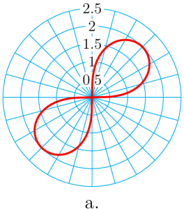
Finally, change [latex]\theta\text{ max}[/latex] to [latex]\pi\text{,}[/latex] and graph again. For [latex]\theta[/latex] between [latex]\dfrac{2\pi}{3}[/latex] and [latex]\pi\text{,}[/latex] the graph traces out a third loop, as shown in figure (c). For [latex]\theta[/latex] between [latex]\pi[/latex] and [latex]2\pi\text{,}[/latex] the entire graph is traced a second time. The finished graph is a rose with 3 petals of length 2.
Checkpoint 10.22.
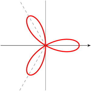
Use your calculator to graph the polar equation [latex]r=2\cos 3\theta\text{.}[/latex]
Complete the table of values for the function.
[latex]\theta[/latex]
[latex]0[/latex]
[latex]\dfrac{\pi}{6}[/latex]
[latex]\dfrac{\pi}{3}[/latex]
[latex]\dfrac{\pi}{2}[/latex]
[latex]\dfrac{2\pi}{3}[/latex]
[latex]\dfrac{5\pi}{6}[/latex]
[latex]\pi[/latex]
[latex]r[/latex]
[latex]\hphantom{000}[/latex]
[latex]\hphantom{000}[/latex]
[latex]\hphantom{000}[/latex]
[latex]\hphantom{000}[/latex]
[latex]\hphantom{000}[/latex]
[latex]\hphantom{000}[/latex]
[latex]\hphantom{000}[/latex]
Sketch the graph by hand on the grid at right.
Solution
Sketching Familiar Equations
You should also be able to sketch the standard polar graphs by hand. Once you recognize an equation as a particular type of graph, say a rose or a limaçon, you can sketch the graph quickly by finding just a few well-chosen guide points. The next example demonstrates a technique for sketching a rose.
Example 10.23.
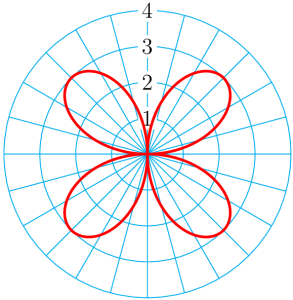
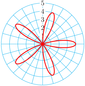
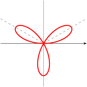
Graph the polar equation [latex]r=3\sin 2\theta\text{.}[/latex]
Solution
Referring to the Catalog of Polar Graphs, we see that the graph of this equation is a rose, with petal length [latex]a=3[/latex] and four petals, because [latex]2n=4\text{.}[/latex] If we can locate the tips of the petals, we can use them as guide points to sketch the graph.
Now, the points at the tips of the petals have [latex]r=3\text{,}[/latex] so we substitute [latex]r=3[/latex] into the equation of the rose to find the values of [latex]\theta[/latex] at those points.
[latex]3 =3\sin 2\theta \qquad \text{Divide both sides by 3.}[/latex]
[latex]1 = \sin 2\theta \qquad ~~ \text{Apply the arcsine function to both sides.}[/latex]
[latex]\dfrac{\pi}{2} = 2\theta \qquad ~~~~~~ \text{Divide both sides by 2.}[/latex]
[latex]\dfrac{\pi}{4} = \theta[/latex]
Thus, one of the petal tips is located at [latex]\theta = \dfrac{\pi}{4}\text{.}[/latex] Because the 4 petals are evenly spaced around the pole, the angle between the petals is [latex]\dfrac{2\pi}{4} = \dfrac{\pi}{2}\text{,}[/latex] and the other petal tips occur at
We plot the tips of the petals as guide points, at [latex]\left(3, \dfrac{\pi}{4}\right)\text{,}[/latex][latex]~ \left(3, \dfrac{3\pi}{4}\right)\text{,}[/latex] [latex]~ \left(3, \dfrac{5\pi}{4}\right)[/latex]and [latex](3, \dfrac{7\pi}{4})\text{.}[/latex] Now we can sketch a rose with 4 petals of length 3, as shown at right.
Checkpoint 10.24.
Graph the polar equation [latex]r=4\cos 5\theta\text{.}[/latex]
Solution
The limaçons, [latex]r=a\pm\sin \theta[/latex] and [latex]r=a\pm\cos \theta\text{,}[/latex] are another family of polar graphs. In particular, the cardioid is a special case of a limaçon with [latex]a=b\text{.}[/latex]
Example 10.25.
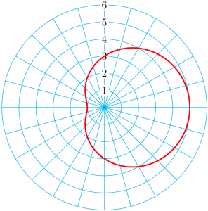
Graph the polar equation [latex]r=3+2\cos \theta\text{.}[/latex]
Solution
This is the equation for a limaçon, with [latex]a=3[/latex] and [latex]b=2\text{.}[/latex] Because [latex]a \gt b\text{,}[/latex] the limaçon will have a dent, like a lima bean, rather than a loop. As guide points, we locate the points at the four quadrantal angles.
[latex]\theta[/latex]
[latex]r=3+2\cos\theta[/latex]
[latex]0[/latex]
[latex]5[/latex]
[latex]\dfrac{\pi}{2}[/latex]
[latex]3[/latex]
[latex]\pi[/latex]
[latex]1[/latex]
[latex]\dfrac{3\pi}{2}[/latex]
[latex]3[/latex]
We plot the guide points and connect them in order with a smooth curve, as shown below. Note that this limaçon involving cosine is symmetric about the [latex]x[/latex]-axis; limaçons involving sine are symmetric about the [latex]y[/latex]-axis.
Checkpoint 10.26.
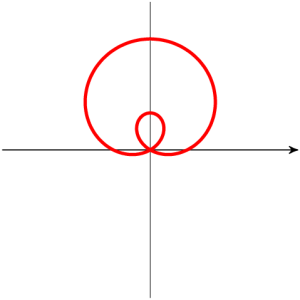
Graph the polar equation [latex]r=1-3\sin \theta\text{.}[/latex]
Solution
You should also be able to identify a polar graph and write its equation.
Example 10.27.
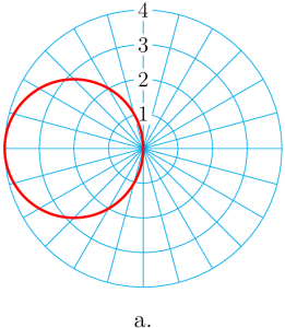
Give a polar equation for each of the graphs below.
Solution
The graph is a circle centered at [latex](-2,0)[/latex] and with radius 2, so we choose the equation [latex]r=2a\cos \theta\text{,}[/latex] with [latex]a=-2\text{.}[/latex] Thus, [latex]r=-4\cos \theta\text{.}[/latex]
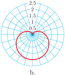
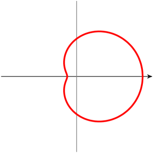
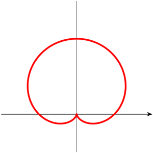
The graph is a cardioid with its axis of symmetry on the [latex]x[/latex]-axis, and the "bottom" of the heart points in the positive[latex]x[/latex]direction, so its equation has the form [latex]r=a+a\cos \theta\text{.}[/latex] At [latex]\theta=0,~ r=2\text{,}[/latex] so we can solve for [latex]a\text{:}[/latex][latex]2 = a + a\cos 0\\ 2 = a + a(1) =2a[/latex]Thus, [latex]a=1[/latex] and we choose the equation [latex]r=1+\cos \theta\text{.}[/latex]
Checkpoint 10.28.
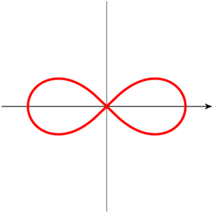
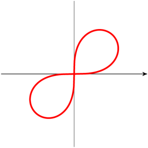
Give a polar equation for each of the graphs below.
Solution
[latex]\displaystyle r^2=4\sin 2\theta[/latex]
[latex]\displaystyle r=1-\sin \theta[/latex]
Finding Intersection Points
To find the intersection points of two graphs, we solve the system made up of their equations. If the equations are [latex]y=f(x)[/latex] and [latex]y=g(x)\text{,}[/latex] we simply solve the equation [latex]f(x)=g(x)\text{.}[/latex] For example, we find the intersection points of [latex]y=x^2[/latex] and [latex]y=x+2[/latex] by solving the equation [latex]x^2-x-2=0[/latex] to get
These are the [latex]x[/latex]-coordinates of the intersection points, and we can find the [latex]y[/latex]-coordinates by substituting these values into either equation.
For [latex]x=2,[/latex] we find [latex]y=2^2=4.[/latex]
For [latex]x=-1,[/latex] we find [latex]y=(-1)^2=1.[/latex]
Thus, the intersection points are [latex](2,4)[/latex] and [latex](-1,1)\text{,}[/latex] as shown at right.
To find the intersection points of the polar graphs [latex]r=f(\theta)[/latex] and [latex]r=g(\theta)[/latex] we solve the equation [latex]f(\theta) = g(\theta)\text{.}[/latex]
Example 10.29.
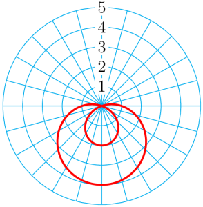
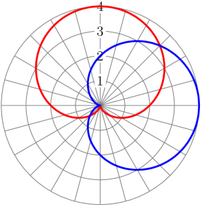
Find all intersection points of the graphs of [latex]~~r=2+2\sin \theta~~[/latex] and [latex]~~r=2+2\cos \theta\text{.}[/latex]
Solution
We equate the two expressions for [latex]r[/latex] and solve for [latex]\theta\text{.}[/latex]
[latex]r=2+2\sin \theta \text{ and } r=2+2\cos \theta[/latex]
[latex]\sin \theta = \cos \theta \qquad \text{Divide both sides by} \cos\theta.[/latex]
[latex]\tan \theta = 1 \qquad \text{Solve for } \theta.[/latex]
[latex]\theta = \dfrac{\pi}{4},~\dfrac{5\pi}{4}[/latex]
We evaluate either expression for [latex]t[/latex] to find the other coordinate of the intersection point.
Thus, two of the intersection points are [latex]\left(2 + \sqrt{2}, \dfrac{\pi}{4}\right)[/latex] and [latex]\left(2 - \sqrt{2}, \dfrac{5\pi}{4}\right)\text{,}[/latex] as shown. However, you can see in the figure that the graphs also appear to intersect at the pole. To verify that the pole indeed lies on both graphs, we can solve for [latex]\theta[/latex] in each equation when [latex]r=0\text{.}[/latex]
However, you can see in the figure that the graphs also appear to intersect at the pole. To verify that the pole indeed lies on both graphs, we can solve for [latex]\theta[/latex] in each equation when [latex]r={0}\text{.}[/latex]
Both points, [latex]\left(0,\dfrac{3\pi}{2}\right)[/latex] and [latex](0,\pi)\text{,}[/latex] represent the pole. Thus, the graphs intersect at three points: [latex]\left(2 + \sqrt{2}, \dfrac{\pi}{4}\right)\text{,}[/latex] [latex]\left(2 - \sqrt{2}, \dfrac{5\pi}{4}\right)\text{,}[/latex] and the pole.
Caution 10.30.
As we saw in the previous example, solving a system of equations [latex]r=f(\theta)[/latex] and [latex]r=g(\theta)[/latex] will not always reveal an intersection at the pole, because [latex]r[/latex] may be equal to zero for different values of [latex]\theta[/latex] in the two equations. We should always check separately whether the pole is a point on both graphs.
Checkpoint 10.31.
Find all intersection points of the graphs of [latex]r=1[/latex] and [latex]r=2\cos\theta\text{.}[/latex]
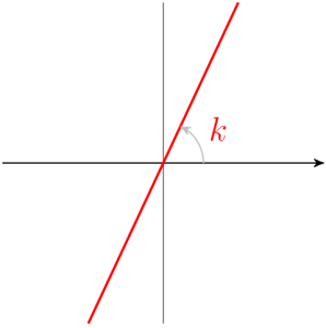
[latex]\theta = k~~[/latex] ([latex]k[/latex] a constant) A line through the pole.
[latex]k[/latex] gives the angle of inclination of the line (in radians).
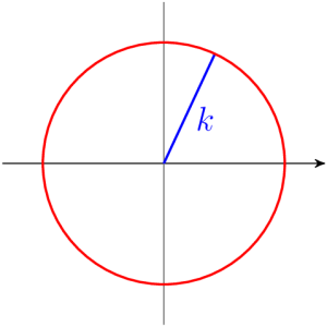
[latex]r = k~~[/latex] ([latex]k[/latex] a constant) A circle centered at the pole.
[latex]k[/latex] is the radius of the circle.
Circles
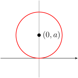
[latex]r=2a\sin \theta[/latex] A circle with center [latex](0,a)[/latex] on the [latex]y[/latex]-axis, and radius [latex]{|a|}\text{.}[/latex]
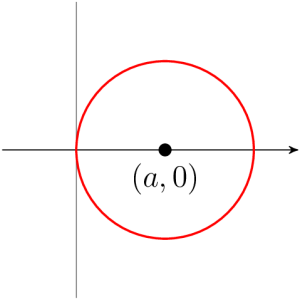
[latex]r=2a\cos \theta[/latex] A circle with center [latex](a,0)[/latex] on the [latex]x[/latex]-axis, and radius [latex]{|a|}\text{.}[/latex]
Roses
[latex]r=a\sin n\theta[/latex] A rose with petal length [latex]a\text{.}[/latex][latex]n[/latex] petals if [latex]n[/latex] is odd; [latex]~~2n[/latex] petals if [latex]n[/latex] is even.
[latex]r=a\cos n\theta[/latex] A rose with petal length [latex]a\text{.}[/latex][latex]n[/latex] petals if [latex]n[/latex] is odd; [latex]~~2n[/latex] petals if [latex]n[/latex] is even.
Limaçons
[latex]r=a\pm b\sin \theta~~~~~[/latex] or [latex]~~~~~r=a\pm b\cos \theta[/latex]
When graphing an equation in polar coordinates, we think of sweeping around the pole in the counterclockwise direction, and at each angle [latex]\theta[/latex] the [latex]r[/latex]-value tells us how far the graph is from the pole.
Standard graphs in polar coordinates include circles and roses, cardioids and limaçons, lemniscates, and spirals.
To find the intersection points of the polar graphs [latex]r=f(\theta)[/latex] and [latex]r=g(\theta)[/latex] we solve the equation [latex]f(\theta)=g(\theta)\text{.}[/latex] In addition, we should always check whether the pole is a point on both graphs.
Study Questions
Delbert says that the graph of [latex]r=2\sin \theta[/latex] in the first example cannot be correct, because there are no points on the graph for angles between [latex]\pi[/latex] and [latex]2\pi\text{.}[/latex] How do you respond?
Is it possible to have a rose with only two petals? What would its equation be?
Francine says that a circle of the form [latex]r=2a\cos \theta[/latex] is just a special case of a limaçon. Support or refute her statement.
There are no points on the graph of [latex]r^2=4\cos 2\theta[/latex] for angles between [latex]\dfrac{\pi}{4}[/latex] and [latex]\dfrac{3\pi}{4}[/latex] Why is that?
Media Attributions
exer10-2-1ans
exam10-2-2
exer10-2-2ans
exam10-2-3a
exam10-2-3b
exam10-2-3c
exer10-2-3
exam10-2-4
exer10-2-4ans
exam10-2-5
exer10-2-5ans
exam10-2-6a
exam10-2-6b
exer10-2-6a
exer10-2-6b
exam10-2-7
cat10-2-1
cat10-2-2
cat10-2-3
at10-2-4
cat10-2-5
cat10-2-6
cat10-2-7
cat10-2-8
cat10-2-9
cat10-2-10
cat10-2-11
cat10-2-12
cat10-2-13
definition
\[ r = a \sin {n\theta} \] or
\[ r = a \cos {n\theta} \]
A limaçon is a curve that can take on various forms, from loops to dimples to heart-like shapes, depending on the values of its parameters
[latex]r=apm bsin theta~[/latex] or [latex]~r=apm bcos theta[/latex]
A cardioid is defined in the polar coordinate system by the equation:
\[ r = a * (1 + \cos( \theta)) \]
[latex]r^2=a^2 cos 2theta[/latex]
[latex]r^2=a^2 sin 2theta[/latex]
A lemniscate graph is a type of mathematical curve which resembles a figure-eight or an infinity symbol [latex]\infty[/latex]