7.2 The General Sinusoidal Function
Algebra Refresher
- Write a formula for [latex]g(x){.}[/latex]
- Graph [latex]f(x)[/latex] and [latex]g(x)[/latex] on the same axes.
- [latex]\displaystyle f(x)=x^2,~g(x)=f(x-2)[/latex]
- [latex]\displaystyle f(x)=\sqrt{x},~g(x)=f(x+4)[/latex]
- [latex]\displaystyle f(x)=\dfrac{1}{x},~g(x)=f(x+1)[/latex]
- [latex]\displaystyle f(x)=\dfrac{1}{x^2},~g(x)=f(x-1)[/latex]
- [latex]\displaystyle f(x)=\lvert {x} \rvert,~g(x)=f(x-3)[/latex]
- [latex]\displaystyle f(x)=2^x,~g(x)=f(x+3)[/latex]
Algebra Refresher Answers
- [latex]\displaystyle g(x)=(x-2)^2[/latex]

- [latex]\displaystyle g(x)=\sqrt{x+4}[/latex]

- [latex]\displaystyle g(x)=\dfrac{1}{x+1}[/latex]

- [latex]\displaystyle g(x)=\dfrac{1}{(x-1)^2}[/latex]

- [latex]\displaystyle g(x)=\\vert {x-3} \rvert[/latex]

- [latex]\displaystyle g(x)=2^{x+3}[/latex]

- Graph trigonometric functions using a table of values
- Find a formula for a transformation of a trigonometric function
- Solve trigonometric equations graphically
- Model periodic phenomena with trigonometric functions
- Fit a circular function to data
Horizontal Shifts
In the previous section, we considered transformations of sinusoidal graphs, including vertical shifts, which change the midline of the graph; vertical stretches and compressions, which change its amplitude; and horizontal stretches and compressions, which occur when we change the period of the graph.
In this section, we consider one more transformation: shifting the graph horizontally. The figure below shows four different transformations of the graph of [latex]y=\sin x{.}[/latex]


Graph [latex]f(x)=\sin x[/latex] and [latex]g(x)= \sin \left(x - \dfrac{\pi}{4}\right)[/latex] in the ZTrig window. How is the graph of [latex]g[/latex] different from the graph of [latex]f{?}[/latex]
Solution
The graphs are shown below. The graph of [latex]g(x)= \sin (x - \dfrac{\pi}{4})[/latex] has the same amplitude, midline, and period as the graph of [latex]f(x)=\sin x{,}[/latex] but the graph of [latex]g[/latex] is shifted to the \right by [latex]\dfrac{\pi}{4}[/latex] units, compared to the graph of [latex]f{.}[/latex]
 We can see why this shift occurs by studying a table of values for the two functions.
| [latex]x[/latex] |
[latex]0[/latex] |
[latex]\dfrac{\pi}{4}[/latex] |
[latex]\dfrac{\pi}{2}[/latex] |
[latex]\dfrac{3\pi}{4}[/latex] |
[latex]\pi[/latex] |
[latex]\dfrac{5\pi}{4}[/latex] |
[latex]\dfrac{3\pi}{2}[/latex] |
[latex]\dfrac{7\pi}{4}[/latex] |
[latex]2\pi[/latex] |
| [latex]f(x)[/latex] |
[latex]0[/latex] |
[latex]\dfrac{sqrt{2}}{2}[/latex] |
[latex]1[/latex] |
[latex]\dfrac{sqrt{2}}{2}[/latex] |
[latex]0[/latex] |
[latex]\dfrac{-sqrt{2}}{2}[/latex] |
[latex]-1[/latex] |
[latex]\dfrac{-sqrt{2}}{2}[/latex] |
[latex]0[/latex] |
| [latex]g(x)[/latex] |
[latex]\dfrac{-sqrt{2}}{2}[/latex] |
[latex]0[/latex] |
[latex]\dfrac{sqrt{2}}{2}[/latex] |
[latex]1[/latex] |
[latex]\dfrac{sqrt{2}}{2}[/latex] |
[latex]0[/latex] |
[latex]\dfrac{-sqrt{2}}{2}[/latex] |
[latex]-1[/latex] |
[latex]\dfrac{-sqrt{2}}{2}[/latex] |
Notice that in the table, [latex]g[/latex] has the same function values as [latex]f{,}[/latex] but each one is shifted [latex]\dfrac{\pi}{4}[/latex] units to the right. The same thing happens in the graph: each [latex]y[/latex]-value appears [latex]\dfrac{\pi}{4}[/latex] units farther to the right on [latex]g[/latex] than it does on [latex]f{.}[/latex]
Checkpoint 7.15.
Graph [latex]f(x)=\cos x[/latex] and [latex]g(x)= \cos \left(x + \dfrac{\pi}{4}\right)[/latex] in the ZTrig window. How is the graph of [latex]g[/latex] different from the graph of [latex]f{?}[/latex]
Solution
The graph of [latex]g[/latex] is shifted [latex]\dfrac{\pi}{4}[/latex] units to the \left of [latex]f{.}[/latex]
The examples above illustrate the following principle.
The graphs of
[latex]y = \sin (x-h)~~~~ {and}~~~~ t = \cos (x-h)[/latex]
are shifted horizontally compared to the graphs of [latex]y = \sin x[/latex] and [latex]y = \cos x{.}[/latex]
- If [latex]h \gt 0{,}[/latex] the graph is shifted to the \right.
- If [latex]h \lt 0{,}[/latex] the graph is shifted to the \left.
We can use a table of values to sketch graphs that involve horizontal shifts.
Make a table of values and sketch a graph of [latex]y=-2\cos \left(x+\dfrac{\pi}{3}\right){.}[/latex]
Solution
First notice that we can write the equation as
[latex]y=-2\cos \left[x-\left(\dfrac{-\pi}{3}\right)\right][/latex]
so that [latex]h = -\dfrac{\pi}{3}{,}[/latex] and we expect the graph to be shifted [latex]\dfrac{\pi}{3}[/latex] units to the \left compared to the graph of [latex]y = \cos x{.}[/latex]
We choose convenient values for the inputs of the cosine function; namely, [latex]x+\dfrac{\pi}{3}{.}[/latex]
| [latex]x[/latex] |
[latex]x+\dfrac{\pi}{3}[/latex] |
[latex]\cos\left(x+\dfrac{\pi}{3}\right)[/latex] |
[latex]y = \cos\left(x+\dfrac{\pi}{3}\right)[/latex] |
|
[latex]{0}[/latex] |
|
|
|
[latex]{\dfrac{\pi}{2}}[/latex] |
|
|
|
[latex]{\pi}[/latex] |
|
|
|
[latex]{\dfrac{3\pi}{2}}[/latex] |
|
|
|
[latex]{2\pi}[/latex] |
|
|
From those values, we work backward to [latex]x[/latex] and forwards to [latex]y{.}[/latex] (To obtain the values of [latex]x{,}[/latex] we subtract [latex]\dfrac{\pi}{3}[/latex]from the values of [latex]x+\dfrac{\pi}{3}{.}[/latex])
| [latex]x[/latex] |
[latex]x+\dfrac{\pi}{3}[/latex] |
[latex]\cos\left(x+\dfrac{\pi}{3}\right)[/latex] |
[latex]y = \cos\left(x+\dfrac{\pi}{3}\right)[/latex] |
| [latex]\dfrac{-\pi}{3}[/latex] |
[latex]0[/latex] |
[latex]1[/latex] |
[latex]-2[/latex] |
| [latex]\dfrac{\pi}{6}[/latex] |
[latex]\dfrac{\pi}{2}[/latex] |
[latex]0[/latex] |
[latex]0[/latex] |
| [latex]\dfrac{2\pi}{3}[/latex] |
[latex]\pi[/latex] |
[latex]-1[/latex] |
[latex]2[/latex] |
| [latex]\dfrac{7\pi}{6}[/latex] |
[latex]\dfrac{3\pi}{2}[/latex] |
[latex]0[/latex] |
[latex]0[/latex] |
| [latex]\dfrac{5\pi}{3}[/latex] |
[latex]2\pi[/latex] |
[latex]1[/latex] |
[latex]-2[/latex] |
To make the graph, we’ll scale the [latex]x[/latex]-axis in multiples of [latex]\dfrac{\pi}{6}{.}[/latex] We plot the guide points [latex](x,y)[/latex] from the table, and sketch a sinusoidal graph through the points. One cycle of the graph is shown below. As we expected, the graph is shifted [latex]\dfrac{\pi}{3}[/latex] units to the left compared to the graph of [latex]y = \cos x{.}[/latex]

Checkpoint 7.17.
Complete the table and sketch a graph of [latex]y = -2+\sin\left(x - \dfrac{\pi}{6}\right)[/latex] on the grid below. (Do you expect the graph to be shifted to the left or to the right, compared to the graph of [latex]y = \sin x{?}[/latex])
| [latex]x[/latex] |
[latex]x-\dfrac{\pi}{6}[/latex] |
[latex]\sin\left(x-\dfrac{\pi}{6}\right)[/latex] |
[latex]y = -2+\sin\left(x-\dfrac{\pi}{6}\right)[/latex] |
|
[latex]0[/latex] |
|
|
|
[latex]\dfrac{\pi}{2}[/latex] |
|
|
|
[latex]\pi[/latex] |
|
|
|
[latex]\dfrac{3\pi}{2}[/latex] |
|
|
|
[latex]2\pi[/latex] |
|
|

Solution
| [latex]x[/latex] |
[latex]x-\dfrac{\pi}{6}[/latex] |
[latex]\sin\left(x-\dfrac{\pi}{6}\right)[/latex] |
[latex]y = -2+\sin\left(x-\dfrac{\pi}{6}\right)[/latex] |
| [latex]\dfrac{\pi}{6}[/latex] |
[latex]0[/latex] |
[latex]0[/latex] |
[latex]-2[/latex] |
| [latex]\dfrac{2\pi}{3}[/latex] |
[latex]\dfrac{\pi}{2}[/latex] |
[latex]1[/latex] |
[latex]-1[/latex] |
| [latex]\dfrac{7\pi}{6}[/latex] |
[latex]\pi[/latex] |
[latex]0[/latex] |
[latex]-2[/latex] |
| [latex]\dfrac{5\pi}{3}[/latex] |
[latex]\dfrac{3\pi}{2}[/latex] |
[latex]-1[/latex] |
[latex]-3[/latex] |
| [latex]\dfrac{13\pi}{6}[/latex] |
[latex]2\pi[/latex] |
[latex]0[/latex] |
[latex]-2[/latex] |

The order in which we apply transformations to a function makes a difference in the graph. We’ll compare the graphs of the two functions
[latex]f(x) = \sin [2(x - \dfrac{\pi}{3})]~~~~ {and} ~~~~ g(x)= \sin (2x - \dfrac{\pi}{3})[/latex]
Graph the two functions in the ZTrig window, along with [latex]y = \sin 2x{,}[/latex] as shown below. Each graph involves a horizontal shift relative to [latex]y = \sin 2x{,}[/latex] but the graph of [latex]f[/latex] is shifted [latex]\dfrac{\pi}{3}[/latex] units to the right, while the graph of [latex]g[/latex] is shifted only [latex]\dfrac{\pi}{6}[/latex] units to the right. This difference occurs because of the order of the transformations.


We transform the graph of [latex]y = \sin x[/latex] into the graph of [latex]f[/latex] in two steps:
Step 1: First we replace [latex]x[/latex] by [latex]2x[/latex] to get [latex]y = \sin 2x{,}[/latex] which compresses the graph horizontally by a factor of 2. (See figure [a] below.)
Step 2: Then we replace [latex]x[/latex] by [latex]x - \dfrac{\pi}{3}[/latex] to get [latex]f(x) = \sin \left[2\left(x - \dfrac{\pi}{3}\right)\right]{,}[/latex] which shifts the graph [latex]\dfrac{\pi}{3}[/latex] units to the right. (See figure [b].)


To transform the graph of [latex]y = \sin x[/latex] into the graph of [latex]g{,}[/latex] we perform the two steps in the opposite order:
Step 1: We replace [latex]x[/latex] by [latex]x - \dfrac{\pi}{3}[/latex], which shifts the graph [latex]\dfrac{\pi}{3}[/latex] units to the right. (See figure [a].)
Step 2: Then we replace [latex]x[/latex] by [latex]2x[/latex] to get [latex]g(x)= \sin (2x - \dfrac{\pi}{3})[/latex], which compresses the graph horizontally by a factor of 2, including the horizontal shift. This reduces the horizontal shift from [latex]\dfrac{\pi}{3}[/latex] to [latex]\dfrac{\pi}{6}{.}[/latex] (See figure [b].)


It is easier to analyze the transformations in the function [latex]f[/latex] because we can read the horizontal shift from the formula.
[latex]f(x) = \sin 2\left(x - \dfrac{\pi}{3}\right)[/latex]
where [latex]2[/latex] is the compression factor and [latex]\dfrac{\pi}{3}[/latex] is the horizontal shift.
We can write the formula for [latex]g(x)[/latex] in the same easy-to-analyze form by factoring the input for the sine function:
[latex]g(x) = \sin \left(2x - \dfrac{\pi}{3}\right) = \sin 2\left(x - \dfrac{\pi}{6}\right)[/latex]
In general, if we write the formula for a sinusoidal function in standard form, we can read all the transformations from the constants in the formula.
The graphs of the functions
[latex]{y = A\sin B(x-h) + k}~~~~ {and}~~~~ {y = A\cos B(x-h) + k}[/latex]
are transformations of the sine and cosine graphs.
- The amplitude is [latex]\lvert{A} \rvert {.}[/latex]
- The midline is [latex]y = k{.}[/latex]
- The period is [latex]\dfrac{2\pi}{\lvert {B} \rvert},~~B \not= 0{.}[/latex]
- The horizontal shift is [latex]h[/latex] units to the right if [latex]h[/latex] is positive, and [latex]h[/latex] units to the left if [latex]h[/latex] is negative.
- State the midline, amplitude, period, and horizontal shift for the function
[latex]f(x) = 4\cos (3x+\pi) - 2[/latex]
- Sketch a graph of the function for [latex]-\pi \le x \le \pi{.}[/latex]
Solution
- First, we write the input for the cosine function in factored form:[latex]f(x) = 4\cos 3\left(x+\dfrac{\pi}{3}\right) - 2[/latex] Comparing the formula for [latex]f[/latex] with the standard form, we see that [latex]A=4{,}[/latex] [latex]B=3,~h = \dfrac{-\pi}{3}{,}[/latex] and [latex]k = 2{.}[/latex] Thus, the midline is [latex]y = -2{,}[/latex] the amplitude is [latex]4{,}[/latex] the period is [latex]\dfrac{2\pi}{3}{,}[/latex] and the horizontal shift is [latex]\dfrac{\pi}{3}[/latex] units to the left.
- Use a table of values to locate the guide points for the graph. Begin by choosing convenient values for the input, [latex]3x+\pi{.}[/latex] Then work backward to find values for [latex]x[/latex] and forward to find values for [latex]f(x){.}[/latex]
| [latex]x[/latex] |
[latex]3x[/latex] |
[latex]3x+\pi[/latex] |
[latex]\cos(3x+\pi)[/latex] |
[latex]4\cos 3(x+\dfrac{\pi}{3})-2[/latex] |
| [latex]\dfrac{-\pi}{3}[/latex] |
[latex]-\pi[/latex] |
[latex]0[/latex] |
[latex]1[/latex] |
[latex]2[/latex] |
| [latex]\dfrac{-\pi}{6}[/latex] |
[latex]\dfrac{-\pi}{2}[/latex] |
[latex]\dfrac{\pi}{2}[/latex] |
[latex]0[/latex] |
[latex]-2[/latex] |
| [latex]0[/latex] |
[latex]0[/latex] |
[latex]\pi[/latex] |
[latex]-1[/latex] |
[latex]-6[/latex] |
| [latex]\dfrac{\pi}{6}[/latex] |
[latex]\dfrac{\pi}{2}[/latex] |
[latex]\dfrac{3\pi}{2}[/latex] |
[latex]0[/latex] |
[latex]-2[/latex] |
| [latex]\dfrac{\pi}{3}[/latex] |
[latex]\pi[/latex] |
[latex]2\pi[/latex] |
[latex]1[/latex] |
[latex]2[/latex] |
Finally, plot the guide points and connect them with a sinusoidal curve. The graph is shown at right.

Checkpoint 7.19.
- State the midline, amplitude, period, and horizontal shift of the graph of
[latex]g(x) = 150 - 25\cos \left(4x-\dfrac{\pi}{2}\right)[/latex]
- Make a table of values and sketch a graph of the function.
| [latex]x[/latex] |
[latex]4x[/latex] |
[latex]4x-\dfrac{\pi}{2}[/latex] |
[latex]\cos\left(4x-\dfrac{\pi}{2}\right)[/latex] |
[latex]150 - 25\cos\left(4x-\dfrac{\pi}{2}\right)[/latex] |
| [latex]\hphantom{0000}[/latex] |
[latex]\hphantom{0000}[/latex] |
[latex]0[/latex] |
[latex]\hphantom{0000}[/latex] |
[latex]\hphantom{0000}[/latex] |
| [latex]\hphantom{0000}[/latex] |
[latex]\hphantom{0000}[/latex] |
[latex]\dfrac{\pi}{2}[/latex] |
[latex]\hphantom{0000}[/latex] |
[latex]\hphantom{0000}[/latex] |
| [latex]\hphantom{0000}[/latex] |
[latex]\hphantom{0000}[/latex] |
[latex]\pi[/latex] |
[latex]\hphantom{0000}[/latex] |
[latex]\hphantom{0000}[/latex] |
| [latex]\hphantom{0000}[/latex] |
[latex]\hphantom{0000}[/latex] |
[latex]\dfrac{3\pi}{2}[/latex] |
[latex]\hphantom{0000}[/latex] |
[latex]\hphantom{0000}[/latex] |
| [latex]\hphantom{0000}[/latex] |
[latex]\hphantom{0000}[/latex] |
[latex]2\pi[/latex] |
[latex]\hphantom{0000}[/latex] |
[latex]\hphantom{0000}[/latex] |
Solution
- midline: [latex]y=150{,}[/latex] amplitude: [latex]25{,}[/latex] period: [latex]\dfrac{\pi}{2}{,}[/latex] horizontal shift: [latex]\dfrac{\pi}{8}[/latex] to the right
-
| [latex]x[/latex] |
[latex]4x[/latex] |
[latex]4x-\dfrac{\pi}{2}[/latex] |
[latex]\cos\left(4x-\dfrac{\pi}{2}\right)[/latex] |
[latex]150-25\cos\left(4x-\dfrac{\pi}{2}\right)[/latex] |
| [latex]\dfrac{\pi}{8}[/latex] |
[latex]\dfrac{\pi}{2}[/latex] |
[latex]0[/latex] |
[latex]1[/latex] |
[latex]125[/latex] |
| [latex]\dfrac{\pi}{4}[/latex] |
[latex]\pi[/latex] |
[latex]\dfrac{\pi}{2}[/latex] |
[latex]0[/latex] |
[latex]150[/latex] |
| [latex]\dfrac{3\pi}{8}[/latex] |
[latex]\dfrac{3\pi}{2}[/latex] |
[latex]\pi[/latex] |
[latex]-1[/latex] |
[latex]175[/latex] |
| [latex]\dfrac{\pi}{2}[/latex] |
[latex]2\pi[/latex] |
[latex]\dfrac{3\pi}{2}[/latex] |
[latex]0[/latex] |
[latex]150[/latex] |
| [latex]\dfrac{5\pi}{8}[/latex] |
[latex]\dfrac{5\pi}{2}[/latex] |
[latex]2\pi[/latex] |
[latex]1[/latex] |
[latex]125[/latex] |

In Section 7.1 we found formulas for sinusoidal functions that start on the midline, or at their maximum or minimum value. We use horizontal transformations to write formulas for functions that start at other points on the cycle.
Find a formula for the sinusoidal function whose graph is shown below. 
Solution
The midline of the graph is [latex]y=0{,}[/latex] and its amplitude is [latex]4{.}[/latex] It has the shape of a cosine, but its maximum value occurs at [latex]x=\dfrac{\pi}{6}[/latex] instead of at [latex]x=0{,}[/latex] so the graph is shifted [latex]\dfrac{\pi}{6}[/latex] units to the right compared to the graph of [latex]y=\cos x{.}[/latex]
The graph completes one cycle between [latex]x=\dfrac{\pi}{6}[/latex] and [latex]x=\dfrac{13\pi}{6}{,}[/latex] so its period is [latex]2\pi{.}[/latex] Thus, we use the standard form [latex]y = A\cos B(x-h) + k[/latex] with [latex]A=4,~B=1,~h=\dfrac{\pi}{6}{,}[/latex] and [latex]k=0{,}[/latex] giving us
[latex]y = 4\cos (x-\dfrac{\pi}{6})[/latex]
as our formula for the function.
Checkpoint 7.22.
Find a formula for the sinusoidal function whose graph is shown at right.

Solution
[latex]y = 6\sin \left(x - \dfrac{\pi}{4}\right)[/latex]
Many natural phenomena can be modeled with sinusoidal functions.
Sunspots are dark regions on the Sun first observed by Galileo in 1610. The number of sunspots is not constant but varies with a period of approximately 11 years, called the solar cycle. Solar activity is directly related to this cycle and can cause disturbances in the earth’s upper atmosphere. Planning for satellite orbits and space missions requires knowledge of solar activity levels years in advance. The figure below shows sunspot data for the last solar cycle, from July 1985 through June 1996, and a sinusoidal function that models the data. 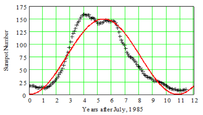
- The period of the solar cycle shown is actually 10.8 years. Use this information and the graph to write a formula for the model.
- Improve the fit of the model by adjusting its horizontal shift.
Solution
- The graph has the shape of [latex]y=-\cos x{.}[/latex] It appears to have midline [latex]y=75[/latex] and amplitude [latex]75{,}[/latex] so [latex]k=75[/latex] and [latex]A=-75[/latex]. To find [latex]B{,}[/latex] we compute
[latex]B=\dfrac{2\pi}{{period}}=\dfrac{2\pi}{10.8}=0.58[/latex]
Thus, a formula for the model is [latex]y=75-75\cos[0.58(x-h)]{.}[/latex]
- Fitting a curve by eye is a subjective process, but it looks like we can get a better fit by shifting the curve slightly to the left. By trying several values for [latex]h[/latex] in [latex]y=75-75\cos[0.58(x-h)]{,}[/latex] we might settle on [latex]h=0.3{,}[/latex] which results in the curve shown below.

Checkpoint 7.24.
The figure below shows the sunspot data for the current solar cycle, which began in July 1996, and a curve of best fit calculated by NASA. This curve is not sinusoidal but has a similar shape.
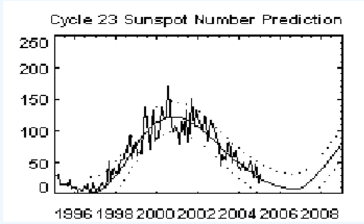
- The minimum sunspot number occurred in October 1996. Use the graph to estimate the period, midline, and amplitude of a sinusoidal function that approximates the data.
- Write a function that approximates the data.
- Use your function to predict the sunspot number in January 2005.
Solution
- Period: 10 years, midline: [latex]y=61.5{,}[/latex] amplitude: 53
- [latex]\displaystyle y=61.5-53\cos (x-0.25)[/latex]
- 37
Concepts
-
Horizontal Shifts.
The graphs of
[latex]y = \sin (x-h)~~~~ {and}~~~~ t = \cos (x-h)[/latex]
are shifted horizontally compared to the graphs of [latex]y = \sin x[/latex] and [latex]y = \cos x{.}[/latex]
- If [latex]h \gt 0{,}[/latex] the graph is shifted to the right.
- If [latex]h \lt 0{,}[/latex] the graph is shifted to the left.
- The order in which we apply transformations to a function makes a difference in the graph.
-
Standard Form for Sinusoidal Functions.
The graphs of the functions
[latex]y = A\sin B(x-h) + k~~~~ {and}~~~~ y = A\cos B(x-h) + k[/latex]
are transformations of the sine and cosine graphs.
- The amplitude is [latex]\lvert {A} \rvert {.}[/latex]
- The midline is [latex]y = k{.}[/latex]
- The period is [latex]\dfrac{2\pi}{\lvert {B} \rvert},~~B \not= 0{.}[/latex]
- The horizontal shift is [latex]h[/latex] units to the right if [latex]h[/latex] is positive, and [latex]h[/latex] units to the left if [latex]h[/latex] is negative.
Study Questions
- Which of the following functions are the same? Explain your answer.
[latex]f(x)=\cos (2x-\dfrac{\pi}{3}), ~~ g(x)=(\cos 2x)-\dfrac{\pi}{3}, ~~ h(x)=\cos 2x - \cos \dfrac{\pi}{3}[/latex]
- Which of the following functions are the same? Explain your answer.
[latex]f(x)=\sin \left(2x-\dfrac{\pi}{3}\right), ~~ g(x)=\sin \left[2\left(x-\dfrac{\pi}{6}\right)\right], ~~ h(x)=2\sin \left(x - \dfrac{\pi}{6})\right)[/latex]
Calculate the horizontal shift.
- [latex]\displaystyle y=-2\sin \left(3x-\dfrac{\pi}{4}\right)[/latex]
- [latex]\displaystyle y=6\cos \left(2x+\dfrac{3\pi}{4}\right)[/latex]
- [latex]\displaystyle y=12\cos \left(\dfrac{t}{3}+0.8\right)[/latex]
- [latex]\displaystyle y=-5\sin \left(\dfrac{t}{4}-0.6\right)[/latex]