Introduction

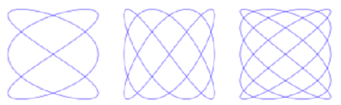
A Lissajous figure is a pattern produced by the intersection of two sinusoidal curves at right angles to each other (Figure 1). They are the curves you often see on oscilloscope screens depicting compound vibration.

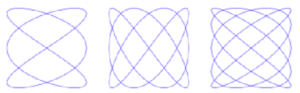
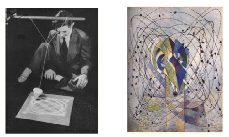
They were first studied by the American mathematician Nathaniel Bowditch in 1815 and later by the French mathematician Jules Antoine Lissajous. Today they have applications in physics and astronomy, medicine, music, and many other fields. In 1855 Lissajous invented a pair of tuning forks designed to visualize sound vibrations. Each tuning fork had a small mirror mounted at the end of one prong, and a light beam reflected from one mirror to the other was projected onto a screen, producing a Lissajous figure. Stable patterns appear only when the two forks vibrate at frequencies in simple ratios, such as 2:1 or 3:2, which correspond to the musical intervals of the octave and perfect fifth. So by observing the Lissajous figures, people were able to make tuning adjustments more accurately than they could do by ear. In 1942 the Dadaist artist Max Ernst punched a small hole in a can of paint, attached it to a coupled pendulum, and set it swinging to create Lissajous figures (Figure 2, left). He then used the designs in some of his paintings (Figure 2, right).

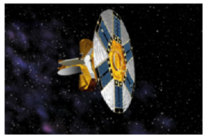
In 2001, NASA launched the Wilkinson Microwave Anisotropy Probe (WMAP) to make fundamental measurements of our universe as a whole (Figure 3). The probe was positioned near a gravitational balance point between Earth and the Sun and moved in a controlled Lissajous pattern around the point. This orbit isolated the spacecraft from radio emissions from Earth.

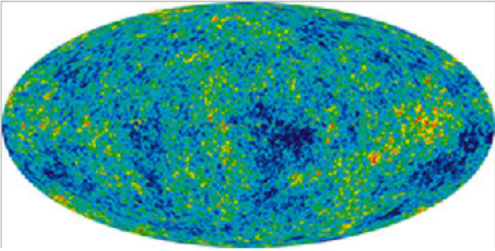
The goal of WMAP was to map the relative cosmic microwave background (CMB) temperature over the full sky. CMB radiation is the radiant heat left over from the big bang. Tiny fluctuations in the CMB are the result of fluctuations in the density of matter in the early universe, so they carry information about the initial conditions for the formation of cosmic structures such as galaxies, clusters, and voids. Here is the first fine-resolution map of the microwave sky, produced from the WMAP data. This picture of the infant universe shows the temperature fluctuations corresponding to the seeds of galaxies (Figure 4).

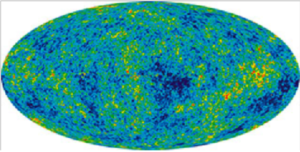
From the WMAP data, scientists were able to do the following:

• Estimate the age of the universe at 13.77 billion years old.
• Calculate the curvature of space to within 0.4% of “flat” Euclidean.
• Determine that ordinary atoms (also called baryons) make up only 4.6% of the universe.
• Find that dark matter (matter not made of atoms) is 24.0% of the universe.

Class Activities