Chapter 6: Radians
Introduction to Trig Radians
Introduction
Have you ever wondered why we divide the circle into 360 degrees? Nobody really knows the answer, but it may well have started around 600 BCE with the Babylonians.
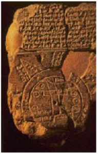
The Babylonians lived between the Tigris and Euphrates rivers in present-day Turkey and Syria. They kept written records using a stylus to press cuneiform, or wedge-shaped, symbols into wet clay tablets, which were then baked in the sun (Figure 1). Thousands of these tablets have survived and give us detailed information about the mathematical practices of the time.
The Babylonians used a base-60 number system because the number 60 has many factors. They did not invent decimal fractions, so they found it difficult to deal with remainders when doing division. But 60 can be divided evenly by 2, 3, 4, 5, and 6, which made calculations with common fractions much easier.
We still see traces of their base-60 system in our own day: there are 60 seconds in a minute, and 60 minutes in an hour.
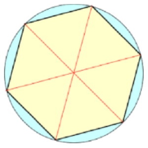
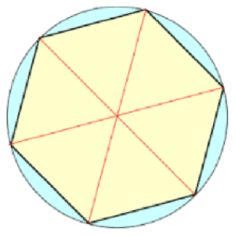
In geometry, Babylonian mathematicians used the corner of an equilateral triangle as their basic unit of angular measure, and naturally divided that angle into 60 smaller angles (Figure 2). Now, if the corners of six equilateral triangles are placed together, they form a complete circle, and that is why there are six times 60, or 360 degrees of arc in a circle.
During the reign of Nebuchadnezzar, using the tools and technology available to them, Babylonian astronomers calculated that a complete year numbered 360 days. This made dividing the circle into 360 degrees even more useful.
So the number 360 is not fundamental to the nature of a circle. If ancient civilizations had defined the full circle to be some other number of degrees, we’d probably be using that number today.
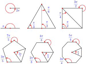
But why do we need another, different way to measure angles? In this chapter we’ll study radian measure, which at first may seem awkward and unnatural (Figure 3). As a hint, consider that although 360 is not fundamental to circles, the number [latex]\pi[/latex] is.
Radians connect the measure of an angle with the arclength it cuts out on a circle.
Imagine a circle of radius 1 unit rolling along a straight line (Figure 4). The circumference of a circle is [latex]2\pi[/latex] times the length of its radius, so when the circle has turned through one complete revolution, it has traveled a distance of [latex]2\pi[/latex] units. When the circle has turned through half a revolution, it has traveled a distance of [latex]\pi[/latex] units.
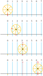
In radian measure, the angle through which the circle has turned is equal to the distance the circle has traveled, or the length of the arc that has unrolled on the line.
The idea of radian measure was developed by Roger Cotes, an English mathematician who worked closely with Isaac Newton. He described the radian in everything but name and recognized its naturalness as a unit of angular measure.
The term radian first appeared in print on June 5, 1873, on an exam written by James Thomson, the brother of Lord Kelvin, at Queen’s College in Belfast.
In calculus and most other branches of mathematics beyond practical geometry, angles are nearly always measured in radians. Because radians arise naturally when dealing with circles, important relationships are expressed more concisely in radians. In particular, results involving trigonometric functions are simpler when the variables are expressed in radians.
Class Activities
Activity 6.2. Radians
Here is a unit circle with arclengths labeled, measured counterclockwise from [latex](1,0){.}[/latex] (Note that the distance around the whole circle is 6.28 units!)

- Use the unit circle to estimate the sine, cosine, and tangent of each angle in radians.
- [latex]0.6[/latex]
- [latex]2.3[/latex]
- [latex]3.5[/latex]
- [latex]5.3[/latex]
- Use the unit circle to estimate two solutions to each equation.
- [latex]\cos t = 0.3[/latex]
- [latex]\sin t = 0.7[/latex]
- Sketch the angle on the unit circle. Find the reference angle in radians, rounded to two decimal places, and sketch the reference triangle.
- [latex]1.8[/latex]
- [latex]5.2[/latex]
- [latex]3.7[/latex]
- Give a decimal approximation to two places for each angle, then the degree measure of each.
Radians [latex]0[/latex] [latex]\dfrac{\pi}{12}[/latex] [latex]\dfrac{\pi}{6}[/latex] [latex]\dfrac{\pi}{4}[/latex] [latex]\dfrac{\pi}{3}[/latex] [latex]\dfrac{5\pi}{12}[/latex] [latex]\dfrac{\pi}{2}[/latex] [latex]\dfrac{7\pi}{12}[/latex] [latex]\dfrac{2\pi}{3}[/latex] [latex]\dfrac{3\pi}{4}[/latex] [latex]\dfrac{5\pi}{6}[/latex] [latex]\dfrac{11\pi}{12}[/latex] [latex]\pi[/latex] Decimal
Approx.[latex]\hphantom{000}[/latex] [latex]\hphantom{000}[/latex] [latex]\hphantom{000}[/latex] [latex]\hphantom{000}[/latex] [latex]\hphantom{000}[/latex] [latex]\hphantom{000}[/latex] [latex]\hphantom{000}[/latex] [latex]\hphantom{000}[/latex] [latex]\hphantom{000}[/latex] [latex]\hphantom{000}[/latex] [latex]\hphantom{000}[/latex] [latex]\hphantom{000}[/latex] [latex]\hphantom{0}[/latex] Degrees [latex]\hphantom{000}[/latex] [latex]\hphantom{000}[/latex] [latex]\hphantom{000}[/latex] [latex]\hphantom{000}[/latex] [latex]\hphantom{000}[/latex] [latex]\hphantom{000}[/latex] [latex]\hphantom{000}[/latex] [latex]\hphantom{000}[/latex] [latex]\hphantom{000}[/latex] [latex]\hphantom{000}[/latex] [latex]\hphantom{000}[/latex] [latex]\hphantom{000}[/latex] [latex]\hphantom{0}[/latex] Radians [latex]\pi[/latex] [latex]\frac{13\pi}{12}[/latex] [latex]\dfrac{7\pi}{6}[/latex] [latex]\dfrac{5\pi}{4}[/latex] [latex]\dfrac{4\pi}{3}[/latex] [latex]\dfrac{17\pi}{12}[/latex] [latex]\dfrac{3\pi}{2}[/latex] [latex]\frac{19\pi}{12}[/latex] [latex]\dfrac{5\pi}{3}[/latex] [latex]\dfrac{7\pi}{4}[/latex] [latex]\frac{11\pi}{6}[/latex] [latex]\frac{23\pi}{12}[/latex] [latex]2\pi[/latex] Decimal
Approx.[latex]\hphantom{0}[/latex] [latex]\hphantom{00}[/latex] [latex]\hphantom{00}[/latex] [latex]\hphantom{00}[/latex] [latex]\hphantom{00}[/latex] [latex]\hphantom{00}[/latex] [latex]\hphantom{00}[/latex] [latex]\hphantom{00}[/latex] [latex]\hphantom{00}[/latex] [latex]\hphantom{00}[/latex] [latex]\hphantom{00}[/latex] [latex]\hphantom{00}[/latex] [latex]\hphantom{0}[/latex] Degrees [latex]\hphantom{0}[/latex] [latex]\hphantom{00}[/latex] [latex]\hphantom{00}[/latex] [latex]\hphantom{00}[/latex] [latex]\hphantom{00}[/latex] [latex]\hphantom{00}[/latex] [latex]\hphantom{00}[/latex] [latex]\hphantom{00}[/latex] [latex]\hphantom{00}[/latex] [latex]\hphantom{00}[/latex] [latex]\hphantom{00}[/latex] [latex]\hphantom{00}[/latex] [latex]\hphantom{0}[/latex] - On the unit circle above, plot the endpoint of each arc in standard position.
- [latex]\dfrac{\pi}{3}[/latex]
- [latex]\dfrac{7\pi}{6}[/latex]
- [latex]\dfrac{7\pi}{4}[/latex]
Activity 6.4. Graphs of Sine and Cosine.
We are going to graph [latex]f(t) = \sin t[/latex] and [latex]g(t) = \cos t[/latex] from their definitions. The unit circle [latex]x^2 + y^2 = 1[/latex] at the left of each grid is marked off in radians. (Each tick mark is [latex]0.1[/latex] radian.) The horizontal [latex]t[/latex]-axis of each grid is also marked in radians.
- Choose a value of [latex]t[/latex] along the horizontal axis of the [latex]f(t) = \sin t[/latex] grid. This value of [latex]t[/latex] represents an angle in radians.
- Now look at the unit circle and find the point [latex]P[/latex] designated by that same angle in radians.
- Measure the vertical (signed) distance that gives the [latex]y[/latex]-coordinate of point [latex]P{.}[/latex]
- At the value of [latex]t[/latex] you chose in step 1, lightly draw a vertical line segment the same length as the [latex]y[/latex]-coordinate of [latex]P{.}[/latex] Put a dot at the top (or bottom) of the line segment.
- Repeat for some more values of [latex]t{.}[/latex] Connect the dots to see the graph of [latex]f(t) = \sin t{.}[/latex]

- Choose a value of [latex]t[/latex] along the horizontal axis of the [latex]g(t) = \cos t[/latex] grid. This value of [latex]t[/latex] represents an angle in radians.
- Now look at the unit circle and find the point [latex]P[/latex] designated by that same angle in radians.
- Measure the horizontal (signed) distance that gives the [latex]x[/latex]-coordinate of point [latex]P{.}[/latex]
- At the value of [latex]t[/latex] you chose in step 1, lightly draw a vertical line segment the same length as the [latex]x[/latex]-coordinate of [latex]P{.}[/latex] Put a dot at the top (or bottom) of the line segment.
- Repeat for some more values of [latex]t{.}[/latex] Connect the dots to see the graph of [latex]g(t) = \cos t{.}[/latex]

Activity 6.5. Solving Equations.

-
-
- Use the graph of [latex]y=\sin t[/latex] to estimate two solutions of the equation [latex]\sin t = 0.65{.}[/latex] Show your solutions on the graph.
- Use the unit circle to estimate two solutions of the equation [latex]\sin t = 0.65{.}[/latex] Show your solutions on the circle.
- Use the graph of [latex]y=\sin t[/latex] to estimate two solutions of the equation [latex]\sin t = -0.2{.}[/latex] Show your solutions on the graph.
- Use the unit circle to estimate two solutions of the equation [latex]\sin t = -0.2{.}[/latex] Show your solutions on the circle.
-

-
-
- Use the graph of [latex]y=\cos t[/latex] to estimate two solutions of the equation [latex]\cos t = 0.15{.}[/latex] Show your solutions on the graph.
- Use the unit circle to estimate two solutions of the equation [latex]\cos t = 0.15{.}[/latex] Show your solutions on the circle.
-
- Use the graph of [latex]y=\cos t[/latex] to estimate two solutions of the equation [latex]\cos t = -0.4{.}[/latex] Show your solutions on the graph.
- Use the unit circle to estimate two solutions of the equation [latex]\cos t = -0.4{.}[/latex] Show your solutions on the circle.
-
Media Attributions
- Chapter 6 Introduction Figure 1 © Trigonometry by Katherine Yoshiwara is licensed under a CC BY-SA (Attribution ShareAlike) license
- Chapter 6 Introduction Figure 2 © Trigonometry by Katherine Yoshiwara is licensed under a CC BY-SA (Attribution ShareAlike) license
- Chapter 6 Introduction Figure 3 © Trigonometry by Katherine Yoshiwara is licensed under a CC BY-SA (Attribution ShareAlike) license
- Chapter 6 Introduction Figure 4 © Trigonometry by Katherine Yoshiwara is licensed under a CC BY-SA (Attribution ShareAlike) license