Chapter 1: Algebra Review
Section 1.7 Exponential Functions
Learning Objectives
By the end of this section, the student should be able to:
- Evaluate exponential functions.
- Find the equation of an exponential function.
- Use compound interest formulas.
- Evaluate exponential functions with base [latex]e.[/latex]
Consider these two companies:
- Company [latex]A[/latex] has [latex]100[/latex] stores and expands by opening [latex]50[/latex] new stores a year.
- Company [latex]B[/latex] has [latex]100[/latex] stores and expands by increasing the number of stores by [latex]50\%[/latex] of their total each year.
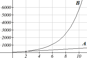
Company [latex]A[/latex] is exhibiting linear growth. In linear growth, we have a constant rate of change – a constant number that the output increased for each increase in input. For company [latex]A[/latex], the number of new stores per year is the same each year.
Company [latex]B[/latex] is different – we have a percent rate of change rather than a constant number of stores/year as our rate of change. To see the significance of this difference, compare a [latex]50\%[/latex] increase when there are [latex]100[/latex] stores to a [latex]50\%[/latex] increase when there are [latex]1000[/latex] stores:
- [latex]100[/latex] stores, a [latex]50%[/latex] increase is [latex]50[/latex] stores in that year.
- [latex]1000[/latex] stores, a [latex]50\%[/latex] increase is [latex]500[/latex] stores in that year.
Calculating the number of stores after several years, we can clearly see the difference in results.
| Years | Company A | Company B |
| [latex]2[/latex] | [latex]200[/latex] | [latex]225[/latex] |
| [latex]4[/latex] | [latex]300[/latex] | [latex]506[/latex] |
| [latex]6[/latex] | [latex]400[/latex] | [latex]1139[/latex] |
| [latex]8[/latex] | [latex]500[/latex] | [latex]2563[/latex] |
| [latex]10[/latex] | [latex]600[/latex] | [latex]5767[/latex] |
This percent growth can be modeled with an exponential function.
Exponential Function
Exponential Growth or Decay Function
An exponential growth or decay function is a function that grows or shrinks at a constant percent growth rate. The equation can be written in the form [latex]f(x)=a(1+r)^x[/latex] or [latex]f(x)=ab^x[/latex] where [latex]b=1+r[/latex].
Where
- [latex]a[/latex] is the initial or starting value of the function;
- [latex]r[/latex] is the percent growth or decay rate, written as a decimal; and
- [latex]b[/latex] is the growth factor or growth multiplier. Since powers of negative numbers behave strangely, we limit [latex]b[/latex] to positive values.
Video
Example 1
India’s population was [latex]1.14[/latex] billion in the year [latex]2008[/latex] and is growing by about [latex]1.34\%[/latex] each year. Write an exponential function for India’s population and use it to predict the population in [latex]2020[/latex].
Using [latex]2008[/latex] as our starting time ([latex]t = 0[/latex]), our initial population will be [latex]1.14[/latex] billion. Since the percent growth rate was [latex]1.34\%[/latex], our value for [latex]r[/latex] is [latex]0.0134[/latex].
Using the basic formula for exponential growth, [latex]f(x)=a(1+r)^x[/latex], we can write the formula [latex]f(t)=1.14(1+0.0134)^{t}.[/latex]
To estimate the population in [latex]2020[/latex], we evaluate the function at [latex]t = 12[/latex], since [latex]2020[/latex] is [latex]12[/latex] years after [latex]2008[/latex]: [latex]f(t)=1.14(1+0.0134)^{12}\approx 1.337 \text{ billion people in 2020.}[/latex]
Example 2
A certificate of deposit (CD) is a type of savings account offered by banks, typically offering a higher interest rate in return for a fixed length of time you will leave your money invested. If a bank offers a [latex]24[/latex]-month CD with an annual interest rate of [latex]1.2\%[/latex] compounded monthly, how much will a [latex]\$1000[/latex] investment grow over those [latex]24[/latex] months? What is the equivalent annual percentage yield ([latex]APY[/latex])?
First, we must notice that the interest rate is an annual rate, but it is compounded monthly, meaning interest is calculated and added to the account monthly. To find the monthly interest rate, we divide the annual rate of [latex]1.2\%[/latex] by [latex]12[/latex], since there are [latex]12[/latex] months in a year: [latex]1.2\%/12 = 0.1\%[/latex]. Each month we will earn [latex]0.1\%[/latex] interest. From this, we can set up an exponential function, with our initial amount of [latex]\$1000[/latex] and a growth rate of [latex]r = 0.001[/latex] and our input [latex]m[/latex] measured in months: [latex]f(m)=1000\left(1+\frac{0.012}{12}\right)^m=1000(1.001)^{m}[/latex]
After [latex]24[/latex] months, the account will have grown to [latex]f(24)=1000(1.001)^{24}\approx \$1024.28[/latex].
The annual percentage yield [latex](APY)[/latex] is the interest rate that is equivalent to [latex]1.2\%[/latex] compounded quarterly if we were to compound annually instead. So we will calculate how much our investment grows in [latex]1[/latex] year (expressed as a percentage of the original amount), which means using [latex]m=12[/latex] months: [latex]f(12)=1000(1.001)^{12}\approx \$1012.07,[/latex] so we have [latex]1012.07/1000=1.01207[/latex] or [latex]101.207\%[/latex] of what we started with, which is a [latex]1.207\%[/latex] gain. Thus our [latex]APY[/latex] is [latex]1.207\%[/latex]. This answer seems reasonable, since when compounding quarterly, we earn interest on interest from the previous quarters, so to compensate for the fact that we are not compounding as often, we need a slightly higher rate to earn an equal amount.
Example 3
Bismuth-210 is an isotope that radioactively decays by about [latex]13\%[/latex] each day, meaning [latex]13\%[/latex] of the remaining Bismuth-210 transforms into another atom (polonium-210, in this case) each day. If you begin with [latex]100[/latex] mg of Bismuth-210, how much remains after one week?
With radioactive decay, instead of the quantity increasing at a percent rate, the quantity is decreasing at a percent rate. Our initial quantity is [latex]a = 100[/latex] mg, and our growth rate will be negative [latex]13\%[/latex], since we are decreasing: [latex]r = -0.13[/latex]. This gives the equation [latex]Q(d)=100(1-0.13)^d=100(0.87)^d.[/latex] This can also be explained by recognizing that if [latex]13\%[/latex] decays, then [latex]87 \%[/latex] remains.
After one week, [latex]7[/latex] days, the quantity remaining would be [latex]Q(7)=100(0.87)^7=37.73[/latex] mg of Bismuth-210 remains.
Example 4
[latex]T(q)[/latex] represents the total number of Android smart phone contracts, in thousands, held by a certain Verizon store region measured quarterly since January 1, 2010. Interpret all of the parts of the equation [latex]T(2)=86(1.64)^2=231.3056[/latex].
Interpreting this from the basic exponential form, we know that [latex]86[/latex] is our initial value. This means that on Jan. 1, 2010, this region had [latex]86,000[/latex] Android smart phone contracts. Since [latex]b = 1 + r = 1.64[/latex], we know that every quarter, the number of smart phone contracts grows by 64%. [latex]T(2) = 231.3056[/latex] means that in the second quarter (or at the end of the second quarter), there were approximately [latex]231,305[/latex] Android smart phone contracts.
When working with exponentials, there is a special constant we must talk about. It arises when we talk about things growing continuously, such as continuous compounding, or natural phenomena like radioactive decay that happen continuously.
Euler’s Number: [latex]e[/latex]
[latex]e\approx 2.718282[/latex]
Because [latex]e[/latex] is often used as the base of an exponential, most scientific and graphing calculators have a button that can calculate powers of [latex]e[/latex], usually labeled e. Some computer software instead defines a function exp(x), where exp(x) = [latex]e^x[/latex]. Since calculus studies continuous change, we will almost always use the [latex]e[/latex]-based form of exponential equations in this course.
Continuous Growth
Continuous Growth Formula
Continuous growth can be calculated using the formula [latex]f(x)=ae^{rx},[/latex] where
- [latex]a[/latex] is the starting amount and
- [latex]r[/latex] is the continuous growth rate.
Example 5
Radon-222 decays at a continuous rate of [latex]17.3\%[/latex] per day. How much will [latex]100[/latex]mg of Radon-222 decay to in [latex]3[/latex] days?
Since we are given a continuous decay rate, we use the continuous growth formula. Since the substance is decaying, we know the growth rate will be negative: [latex]r = -0.173[/latex], [latex]f(3)=100e^{-0.173(3)}\approx 59.512[/latex] mg of Radon-222 will remain.
Graphs of Exponential Functions
Graphical Features of Exponential Functions
Graphically, in the function [latex]f(x)=ab^x[/latex],
- [latex]a[/latex] is the vertical intercept of the graph.
- [latex]b[/latex] determines the rate at which the graph grows:
- the function will increase if [latex]b \gt 1[/latex], and
- the function will decrease if [latex]0 \lt b \lt 1[/latex].
- The graph will have a horizontal asymptote at [latex]y = 0[/latex].
- The graph will be concave up if [latex]a \gt 0[/latex]; concave down if [latex]a \lt 0[/latex].
- The domain of the function is all real numbers.
- The range of the function is [latex](0,\infty)[/latex] if [latex]a \gt 0[/latex], and [latex](-\infty, 0)[/latex] if [latex]a \lt 0[/latex].
When sketching the graph of an exponential function, it can be helpful to remember that the graph will pass through the points [latex](0, a)[/latex] and [latex](1, ab)[/latex].
The value [latex]b[/latex] will determine the function’s long run behavior:
- If [latex]b \gt 1[/latex], as [latex]x\to\infty[/latex], [latex]f(x)\to\infty[/latex], and as [latex]x\to -\infty[/latex], [latex]f(x)\to 0[/latex].
- If [latex]0 \lt b \lt 1[/latex], as [latex]x\to\infty[/latex], [latex]f(x)\to 0[/latex], and as [latex]x\to -\infty[/latex], [latex]f(x)\to \infty[/latex].
Example 6
Sketch a graph of [latex]f(x)=4\left(\frac{1}{3}\right)^x[/latex]
This graph will have a vertical intercept at [latex](0,4)[/latex] and pass through the point [latex]\left(1,\frac{4}{3} \right)[/latex]. Since [latex]b \lt 1[/latex], the graph will be decreasing toward zero. Since [latex]a \gt 0[/latex], the graph will be concave up.
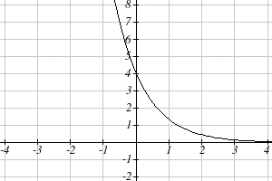
We can also see from the graph the long run behavior: as [latex]x\to\infty[/latex], [latex]f(x)\to 0[/latex], and as [latex]x\to -\infty[/latex], [latex]f(x)\to \infty[/latex].
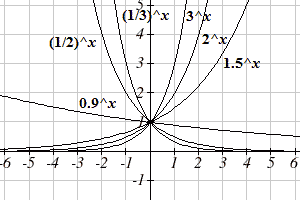
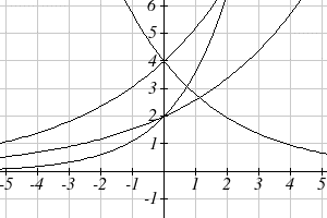
To get a better feeling for the effect of [latex]a[/latex] and [latex]b[/latex] on the graph, examine the sets of graphs below. The first set shows various graphs, where [latex]a[/latex] remains the same and we only change the value for [latex]b[/latex]. Notice that the closer the value of [latex]b[/latex] is to 1, the less steep the graph will be.
In the next set of graphs, [latex]a[/latex] is altered and our value for [latex]b[/latex] remains the same.
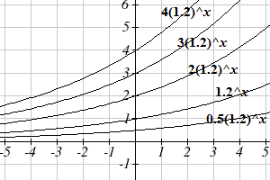
Notice that changing the value for a changes the vertical intercept. Since [latex]a[/latex] is multiplying the [latex]b^x[/latex] term, [latex]a[/latex] acts as a vertical stretch factor, not as a shift. Notice also that the long run behavior for all of these functions is the same because the growth factor did not change and none of these [latex]a[/latex] values introduced a vertical flip.
Try it for yourself using this applet:
Example 7
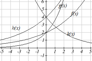
Match each equation with its graph.
- [latex]f(x)=2(1.3)^x[/latex]
- [latex]g(x)=2(1.8)^x[/latex]
- [latex]h(x)=4(1.3)^x[/latex]
- [latex]k(x)=4(0.7)^x[/latex]
The graph of [latex]k(x)[/latex] is the easiest to identify, since it is the only equation with a growth factor of less than one, which will produce a decreasing graph. The graph of [latex]h(x)[/latex] can be identified as the only growing exponential function with a vertical intercept at (0,4). The graphs of [latex]f(x)[/latex] and [latex]g(x)[/latex] both have a vertical intercept at (0,2), but since [latex]g(x)[/latex] has a larger growth factor, we can identify it as the graph increasing faster.
Vocabulary
For any real number x , an exponential function is a function with the form f (x) = ab^x, where
a is a non-zero real number called the initial value and b is any positive real number such that b is not equal to 1.
For all real numbers t , and all positive numbers a and r, continuous growth or decay is represented by the formula A(t) = a e^(rt)
where: a is the initial value, r is the continuous growth rate per unit time, and t is the elapsed time.
If r > 0, then the formula represents continuous growth. If r < 0, then the formula represents continuous decay.
