Chapter 3: Applications of the Derivative
Section 3.4: Other Applications
Learning Objectives
By the end of this section, the student should be able to:
- Use tangent line approximation to solve problems.
- Calculate and interpret elasticity of demand.
Tangent Line Approximation
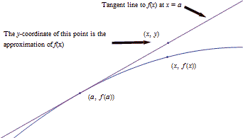
Back when we first thought about the derivative, we used the slope of secant lines over tiny intervals to approximate the derivative: [latex]f'(a)\approx \frac{\Delta y}{\Delta x}=\frac{f(x)-f(a)}{x-a}[/latex]
Now that we have other ways to find derivatives, we can exploit this approximation to go the other way. Solve the expression above for [latex]f(x)[/latex], and you’ll get the tangent line approximation (TLA).
The Tangent Line Approximation (or Linear Approximation
)
To approximate the value of [latex]f(x)[/latex] using TLA, find some [latex]a[/latex] where
- [latex]a[/latex] and [latex]x[/latex] are
close
and - you know the exact values of both [latex]f(a)[/latex] and [latex]f'(a)[/latex].
Then [latex]f(x) \approx f(a)+f'(a)(x-a).[/latex]
Another way to look at the same formula: [latex]\Delta y\approx f'(a)\Delta x[/latex]
How close is close? It depends on the shape of the graph of [latex]f[/latex]. In general, the closer the better.
Video
Example 1
Suppose we know that [latex]g(20) = 5[/latex] and [latex]g'(20) = 1.4[/latex]. Use this information to approximate [latex]g(23)[/latex] and [latex]g(18)[/latex].
Using the tangent line approximation:
[latex]\begin{align*} g(23)= 5 + (1.4)(23 - 20) \approx 9.2\\ g(18)= 5 + (1.4)(18 - 20) \approx 2.2 \end{align*}[/latex]
Note that we don’t know if these approximations are close – but they’re the best we can do with the limited information we have to start with. Note also that 18 and 23 are sort of close to 20, so we can hope these approximations are pretty good. We would feel more confident using this information to approximate [latex]g(20.003)[/latex]. We would feel very unsure using this information to approximate [latex]g(55)[/latex].
Elasticity
We know that demand functions are decreasing, so when the price increases, the quantity demanded goes down. But what about revenue = price [latex]\times[/latex] quantity? When the price increases, will revenue go down because the demand dropped so much? Or will revenue increase because demand didn’t drop very much?
Elasticity of demand is a measure of how demand reacts to price changes. It’s normalized – that means the particular prices and quantities don’t matter, and everything is treated as a percent change. The formula for elasticity of demand involves a derivative, which is why we’re discussing it here.
Elasticity of Demand
Given a demand function that gives [latex]q[/latex] in terms of [latex]p[/latex] (so [latex]q=D(p)[/latex]), the elasticity of demand is
[latex]\begin{align*} E &= \left|\frac{p}{q}\cdot \frac{dq}{dp}\right|\\ &= \left|\frac{p\cdot D'(p)}{D(p)}\right| \end{align*}[/latex]
Note that since demand is (normally) a decreasing function of [latex]p[/latex], the derivative is (normally) negative. That’s why we have the absolute value: so that [latex]E[/latex] will always be positive. This means we can also write [latex]E[/latex] as [latex]-\dfrac{p}{q}\cdot \dfrac{dq}{dp}[/latex] or [latex]-\dfrac{p\cdot D'(p)}{D(p)}[/latex]. These forms can be easier to work with when solving for when [latex]E=1[/latex].
- If [latex]E \lt 1[/latex], we say demand is inelastic. In this case, raising prices increases revenue.
- If [latex]E \gt 1[/latex], we say demand is elastic. In this case, raising prices decreases revenue.
- If [latex]E = 1[/latex], we say demand is unitary. [latex]E = 1[/latex] at critical points of the revenue function.
Interpretation of Elasticity
If the price increases by 1%, the demand will decrease by E%.
Example 2
A company sells [latex]q[/latex] ribbon winders per year at $[latex]p[/latex] per ribbon winder. The demand function for ribbon winders is given by [latex]p=300-0.02q[/latex]. Find the elasticity of demand when the price is $70 apiece. Will an increase in price lead to an increase in revenue?
First, we need to solve the demand equation so it gives [latex]q[/latex] in terms of [latex]p[/latex] so that we can find [latex]\frac{dq}{dp}[/latex]: [latex]p=300-0.02q[/latex], so [latex]q=15000-50p[/latex]. Then [latex]\frac{dq}{dp}=-50[/latex].
We need to find [latex]q[/latex] when [latex]p = 70[/latex]: [latex]q = 11500.[/latex]
Now compute [latex]E=\left| \frac{p}{q}\cdot\frac{dq}{dp} \right|=\left| \frac{70}{11500}\cdot(-50) \right| \approx 0.3[/latex]
[latex]E \lt 1[/latex], so demand is inelastic. Increasing the price by 1% would only cause a 0.3% drop in demand. Increasing the price would lead to an increase in revenue, so it seems that the company should increase its price.
The demand for products that people have to buy, such as onions, tends to be inelastic. Even if the price goes up, people still have to buy about the same amount of onions, and revenue will not go down. The demand for products that people can do without, or put off buying, such as cars, tends to be elastic. If the price goes up, people will just not buy cars right now, and revenue will drop.
Video
Example 3
A company finds the demand [latex]q[/latex], in thousands, for their kites to be [latex]q=400-p^2[/latex] at a price of [latex]p[/latex] dollars. Find the elasticity of demand when the price is $5 and when the price is $15. Then find the price that will maximize revenue.
Calculating the derivative, [latex]\frac{dq}{dp}=-2p[/latex]. The elasticity equation as a function of [latex]p[/latex] will be: [latex]E=\left| \frac{p}{q}\cdot\frac{dq}{dp} \right|=\left| \frac{p}{400-p^2}\cdot (-2p) \right| =\left| \frac{-2p^2}{400-p^2} \right|[/latex]
Evaluating this to find the elasticity at $5 and at $15:
[latex]E = \left| \frac{-2(5)^2}{400-(5)^2} \right| \approx 0.133.[/latex] So the demand is inelastic when the price is $5.
At a price of $5, a 1% increase in price would decrease demand by only 0.133%. Revenue could be raised by increasing prices.
[latex]E = \left| \frac{-2(15)^2}{400-(15)^2} \right| \approx 2.571.[/latex] So the demand is elastic when the price is $15.
At a price of $15, a 1% increase in price would decrease demand by 2.571%. Revenue could be raised by decreasing prices.
To maximize the revenue, we could solve for when [latex]E = 1[/latex]:
[latex]\begin{align*} \left| \frac{-2p^2}{400-p^2} \right|=& 1 \\ 2p^2=& 400-p^2 \\ 3p^2=& 400 \\ p=& \sqrt{\frac{400}{3}}\approx 11.55. \end{align*}[/latex]
A price of $11.55 will maximize the revenue.
Media Attributions
- image099
