Chapter 3: Applications of the Derivative
Section 3.2: Curve Sketching
Learning Objectives
By the end of this section, the student should be able to:
- Use first derivative information to find intervals where graphs are increasing, decreasing, or constant.
- Use second derivative information to determine concavity.
- Use the information about first and second derivatives to graph functions.
This section examines some of the interplay between the shape of the graph of [latex]f[/latex] and the behavior of [latex]f'[/latex]. If we have a graph of [latex]f[/latex], we will see what we can conclude about the values of [latex]f'[/latex]. If we know values of [latex]f'[/latex], we will see what we can conclude about the graph of [latex]f[/latex]. We will also utilize the information from [latex]f''[/latex] that we learned in the last section.
Video
First Derivative Information
Key Takeaways
The function [latex]f(x)[/latex] is increasing on [latex](a,b)[/latex] if [latex]a \lt x_1 \lt x_2 \lt b[/latex] implies [latex]f( x_1 ) \lt f( x_2 )[/latex]. The function [latex]f(x)[/latex] is decreasing on [latex](a, b)[/latex] if [latex]a \lt x_1 \lt x_2 \lt b[/latex] implies [latex]f( x_1 ) \gt f( x_2 )[/latex].
Graphically, [latex]f[/latex] is increasing (decreasing) if, as we move from left to right along the graph of [latex]f[/latex], the height of the graph increases (decreases).
These same ideas make sense if we consider [latex]h(t)[/latex] to be the height (in feet) of a rocket at time [latex]t[/latex] seconds. We naturally say that the rocket is rising or that its height is increasing if the height [latex]h(t)[/latex] increases over a period of time, as [latex]t[/latex] increases.
Example 1
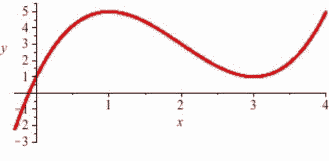
List the intervals on which the function shown is increasing or decreasing.
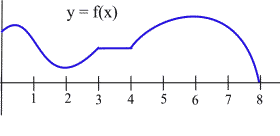
[latex]f[/latex] is increasing on the intervals [0,0.5], [2,3] and [4,6].
[latex]f[/latex] is decreasing on [0.5,2] and [6,8].
On the interval [3,4], the function is not increasing or decreasing; it is constant.
First Derivative Information about Shape (Part 1)
Key Takeaways
For a function [latex]f[/latex] which is differentiable on an interval [latex](a,b)[/latex]:
- If [latex]f[/latex] is increasing on [latex](a,b)[/latex], then [latex]f'(x) \geq 0[/latex] for all [latex]x[/latex] in [latex](a,b)[/latex].
- If [latex]f[/latex] is decreasing on [latex](a,b)[/latex], then [latex]f'(x) \leq 0[/latex] for all [latex]x[/latex] in [latex](a,b)[/latex].
- If [latex]f[/latex] is constant on [latex](a,b)[/latex], then [latex]f'(x) = 0[/latex] for all [latex]x[/latex] in [latex](a,b)[/latex].
Example 2
The graph shows the height of a helicopter during a period of time. Sketch the graph of the upward velocity of the helicopter, [latex]\frac{dh}{dt}[/latex].
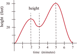
Notice that the [latex]h(t)[/latex] has a local maximum when [latex]t = 2[/latex] and [latex]t = 5[/latex], and so [latex]v(2) = 0[/latex] and [latex]v(5) = 0[/latex]. Similarly, [latex]h(t)[/latex] has a local minimum when [latex]t = 3[/latex], so [latex]v(3) = 0[/latex].
When [latex]h[/latex] is increasing, [latex]v[/latex] is positive. When [latex]h[/latex] is decreasing, [latex]v[/latex] is negative.
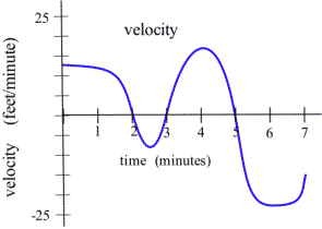
Using this information, we can sketch a graph of [latex]v(t) = \frac{dh}{dt}[/latex].
The next theorem is almost the converse of the first shape theorem and explains the relationship between the values of the derivative and the graph of a function from a different perspective. It says that if we know something about the values of [latex]f'[/latex], then we can draw some conclusions about the shape of the graph of [latex]f[/latex].
First Derivative Information about Shape (Part 2)
Key Takeaways
For a function [latex]f[/latex] which is differentiable on an interval [latex]I[/latex]:
- If [latex]f'(x) \gt 0[/latex] for all [latex]x[/latex] in the interval [latex]I[/latex], then [latex]f[/latex] is increasing on [latex]I[/latex].
- If [latex]f'(x) \lt 0[/latex] for all [latex]x[/latex] in the interval [latex]I[/latex], then [latex]f[/latex] is decreasing on [latex]I[/latex].
- If [latex]f'(x) = 0[/latex] for all [latex]x[/latex] in the interval [latex]I[/latex], then [latex]f[/latex] is constant on [latex]I[/latex].
Example 3
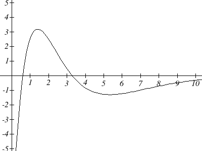
Use information about the values of [latex]f'[/latex] to help graph [latex]f(x) = x^3 - 6x^2 + 9x + 1[/latex]. [latex]f'(x) = 3x^2 - 12x + 9 = 3(x - 1)(x - 3)[/latex], so [latex]f'(x) = 0[/latex] only when [latex]x = 1[/latex] or [latex]x = 3[/latex]. [latex]f'[/latex] is a polynomial, so it is always defined.
The only critical numbers for [latex]f[/latex] are [latex]x = 1[/latex] and [latex]x = 3[/latex], and they divide the real number line into three intervals: [latex](-\infty, 1)[/latex], [latex](1,3)[/latex], and [latex](3, \infty)[/latex]. On each of these intervals, the function is either always increasing or always decreasing.
If [latex]x \lt 1[/latex], then [latex]f '(x) =[/latex] 3(negative number)(negative number) [latex]\gt 0[/latex] so [latex]f[/latex] is increasing.
If [latex]1 \lt x \lt 3[/latex], then [latex]f'(x) =[/latex] 3(positive number)(negative number) [latex]\lt 0[/latex] so f is decreasing.
If [latex]x \gt 3[/latex], then [latex]f'(x) =[/latex] 3(positive number)(positive number) [latex]\gt 0[/latex] so [latex]f[/latex] is increasing.
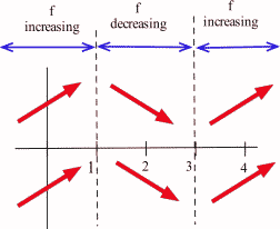
Even though we don’t know the value of [latex]f[/latex] anywhere yet, we do know a lot about the shape of the graph of [latex]f[/latex]: as we move from left to right along the [latex]x[/latex]-axis, the graph of [latex]f[/latex] increases until [latex]x = 1[/latex], then the graph decreases until [latex]x = 3[/latex], and then the graph increases again. The graph of [latex]f[/latex] makes “turns” when [latex]x = 1[/latex] and [latex]x = 3[/latex]; it has a local maximum at [latex]x = 1[/latex] and a local minimum at [latex]x = 3[/latex].
To plot the graph of [latex]f[/latex], we still need to evaluate [latex]f[/latex] at a few values of [latex]x[/latex], but only at a very few values. [latex]f(1) = 5[/latex], and (1,5) is a local maximum of [latex]f[/latex]. [latex]f(3) = 1[/latex], and (3,1) is a local minimum of [latex]f[/latex]. The resulting graph of [latex]f[/latex] is shown here.
Second Derivative Information
Until now, we’ve only used first derivative information, but we could also use information from the second derivative to provide more information about the shape of the function.
Key Takeaways
- If [latex]f[/latex] is concave up on [latex](a,b)[/latex], then [latex]f''(x) \geq 0[/latex] for all [latex]x[/latex] in [latex](a,b)[/latex].
- If [latex]f[/latex] is concave down on [latex](a,b)[/latex], then [latex]f''(x) \leq 0[/latex] for all [latex]x[/latex] in [latex](a,b)[/latex].
The converse of both of these are also true:
- If [latex]f''(x) \geq 0[/latex] for all [latex]x[/latex] in [latex](a,b)[/latex], then [latex]f[/latex] is concave up on [latex](a,b)[/latex].
- If [latex]f''(x) \leq 0[/latex] for all [latex]x[/latex] in [latex](a,b)[/latex], then [latex]f[/latex] is concave down on [latex](a,b)[/latex].
Video
Example 4
Use information about the values of [latex]f''[/latex] to help determine the intervals on which the function [latex]f(x) = x^3 - 6x^2 + 9x + 1[/latex] is concave up and concave down. For concavity, we need the second derivative: [latex]f'(x)=3x^2-12x+9[/latex], so [latex]f''(x)=6x-12[/latex].
To find possible inflection points, set the second derivative equal to zero. [latex]6x-12=0[/latex], so [latex]x = 2[/latex]. This divides the real number line into two intervals: [latex](-\infty,2)[/latex] and [latex](2,\infty)[/latex].
For [latex]x \lt 2[/latex], the second derivative is negative (for example, [latex]f''(0)=6(0)-12=-12[/latex]), so [latex]f[/latex] is concave down. For [latex]x \gt 2[/latex], the second derivative is positive, so [latex]f[/latex] is concave up.
We could have incorporated this concavity information when sketching the graph for the previous example, and indeed we can see the concavity reflected in the graph shown.
Video
Example 5
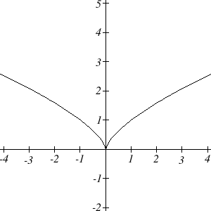
Use information about the values of [latex]f'[/latex] and [latex]f''[/latex] to help graph [latex]f(x)=x^{2/3}[/latex]. [latex]f'(x)=\frac{2}{3}x^{-1/3}[/latex]. This is undefined at [latex]x = 0[/latex].
[latex]f''(x)=-\frac{2}{9}x^{-4/3}[/latex]. This is also undefined at [latex]x = 0[/latex].
This creates two intervals: [latex]x \lt 0[/latex] and [latex]x \gt 0[/latex].
On the interval [latex]x \lt 0[/latex], we could test out a value like [latex]x = -1[/latex]: [latex]f'(-1)=\frac{2}{3}(-1)^{-1/3}=-\frac{2}{3}[/latex] and [latex]f''(-1)=-\frac{2}{9}(-1)^{-4/3}=-\frac{2}{9}.[/latex]
[latex]f'(x)[/latex] is negative and [latex]f''(x)[/latex] is negative, so we can conclude that the function is decreasing and concave down on this interval.
On the interval [latex]x \gt 0[/latex], we could test out a value like [latex]x = 1[/latex]: [latex]f'(1)=\frac{2}{3}(1)^{-1/3}=\frac{2}{3}[/latex] and [latex]f''(1)=-\frac{2}{9}(1)^{-4/3}=-\frac{2}{9}.[/latex]
[latex]f'(x)[/latex] is positive and [latex]f''(x)[/latex] is negative, so we can conclude that the function is increasing and concave down on this interval.
We can also calculate that [latex]f(0)=0[/latex], giving us a base point for the graph. Using this information, we can conclude the graph must look like this:
Video
Sketching without an Equation
Of course, graphing calculators and computers are great at graphing functions. Calculus provides a way to illuminate what may be hidden or out of view when we graph using technology. More importantly, calculus gives us a way to look at the derivatives of functions for which there is no equation given. We already saw the idea of this back in Section 2.3 The Power and Sum Rules for Derivatives, where we sketched the derivative of two graphs by estimating slopes on the curves.
We can summarize all the derivative information about shape in the following table.
Key Takeaways
Summary of Derivative Information about the Graph
| [latex]f(x)[/latex] | Increasing | Decreasing | Concave Up | Concave Down |
| [latex]f'(x)[/latex] | [latex]+[/latex] | [latex]-[/latex] | Increasing | Decreasing |
| [latex]f''(x)[/latex] | [latex]+[/latex] | [latex]-[/latex] |
When [latex]f'(x) = 0[/latex], the graph of [latex]f[/latex] may have a local max or min.
When [latex]f''(x) = 0[/latex], the graph of [latex]f[/latex] may have an inflection point.
Example 6
A company’s bank balance, [latex]B[/latex], in millions of dollars, [latex]t[/latex] weeks after releasing a new product is shown in the graph below. Sketch a graph of the marginal balance – the rate at which the bank balance was changing over time.
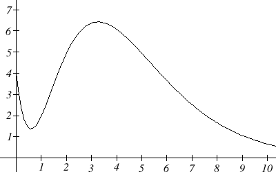
Notice that since the tangent line will be horizontal at about [latex]t = 0.6[/latex] and [latex]t = 3.2[/latex], the derivative will be 0 at those points.
We can then identify intervals on which the original function is increasing or decreasing. This will tell us when the derivative function is positive or negative.
| Interval | [latex]B(t)[/latex] | [latex]B'(t)[/latex] |
| [latex]0 \lt t \lt 0.6[/latex] | Decreasing | Negative |
| [latex]0.6 \lt t \lt 3.2[/latex] | Increasing | Positive |
| [latex]t \gt 3.2[/latex] | Decreasing | Negative |
There appear to be inflection points at about [latex]t =1.5[/latex] and [latex]t = 5.5[/latex]. At these points, the derivative will be changing from increasing to decreasing or vice versa, so the derivative will have a local max or min at those points.
Looking at the intervals of concavity:
| Interval | [latex]B(t)[/latex] | [latex]B'(t)[/latex] |
| [latex]0 \lt t \lt 1.5[/latex] | Concave Up | Increasing |
| [latex]1.5 \lt t \lt 5.5[/latex] | Concave Down | Decreasing |
| [latex]t \gt 5.5[/latex] | Concave Up | Increasing |
If we wanted a more accurate sketch of the derivative function, we could also estimate the derivative at a few points:
| [latex]t[/latex] | [latex]B'(t)[/latex] |
| 0 | -10 |
| 1.5 | 3 |
| 6 | -1 |
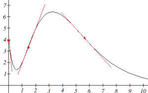
Now we can sketch the derivative. We know a few values for the derivative function, and on each interval we know the shape we need. We can use this to create a rough idea of what the graph should look like.
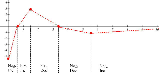
Smoothing this out gives us a good estimate for the graph of the derivative.
Media Attributions
- image072
- image073
- image074
- image075
- image076
- image077
- image078
- image079
- image080
- image081-1
