Chapter 2: Limits and The Derivative
Chapter 2 Review Problems
Review Problems
1.
What is the slope of the line through [latex](3,9)[/latex] and [latex](x, y)[/latex] for [latex]y = x^2[/latex] and [latex]x = 2.97?, \ x = 3.001?, \ x = 3+h[/latex]? What happens to this last slope when h is very small (close to [latex]0[/latex])?
2.
What is the slope of the line through [latex](–2,4)[/latex] and [latex](x, y)[/latex] for [latex]y = x^2[/latex] and [latex]x = –1.98?, \ x = –2.03?, \ x = –2+h[/latex]? What happens to this last slope when h is very small (close to [latex]0[/latex])?
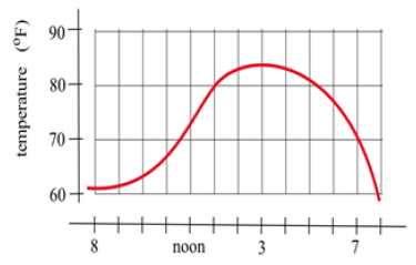
3.
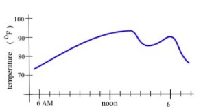
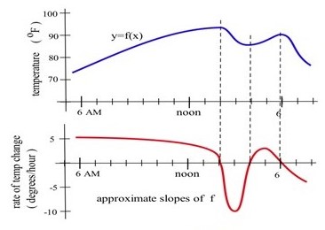
Fig. 36 shows the temperature during a day in Ames.
(a) What was the average change in temperature from [latex]9[/latex] am to [latex]1[/latex] pm?
(b) Estimate how fast the temperature was rising at [latex]10[/latex] am and at [latex]7[/latex] pm.
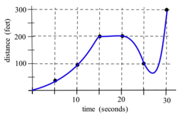
4.
Fig. 37 shows the distance of a car from a measuring position located on the edge of a straight road.
(a) What was the average velocity of the car from [latex]t = 0[/latex] to [latex]t = 30[/latex] seconds?
(b) What was the average velocity of the car from [latex]t = 10[/latex] to t = 30 seconds?
(c) About how fast was the car traveling at [latex]t = 10[/latex] seconds? At [latex]t = 20[/latex] s? At [latex]t = 30[/latex] s?
(d) What does the horizontal part of the graph between [latex]t = 15[/latex] and [latex]t = 20[/latex] seconds mean?
(e) What does the negative velocity at [latex]t = 25[/latex] represent?
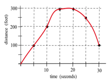
5.
Fig. 38 shows the distance of a car from a measuring position located on the edge of a straight road.
(a) What was the average velocity of the car from [latex]t = 0[/latex] to [latex]t = 20[/latex] seconds?
(b) What was the average velocity from [latex]t = 10[/latex] to [latex]t = 30[/latex] seconds?
(c) About how fast was the car traveling at [latex]t = 10[/latex] seconds? At [latex]t = 20[/latex] s? At [latex]t = 30[/latex] s?
6.
Use the function in Fig. 39 to fill in the table and then graph [latex]m(x)[/latex].
| x | y= f(x) | m(x) = the estimated slope of tangent line to y= f(x) at the point (x,y) |
|---|---|---|
| 0 | ||
| 0.5 | ||
| 1.0 | ||
| 1.5 | ||
| 2.0 | ||
| 2.5 | ||
| 3.0 | ||
| 3.5 | ||
| 4.0 |
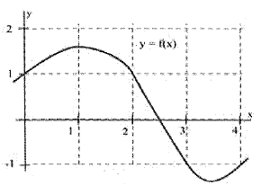
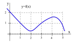
7.
The graph of [latex]y = f(x)[/latex] is given in Fig. 40. Set up a table of values for [latex]x[/latex] and [latex]m(x)[/latex] (the slope of the line tangent to the graph of [latex]y=f(x)[/latex] at the point [latex](x,y)[/latex] ) and then graph the function [latex]m(x)[/latex].
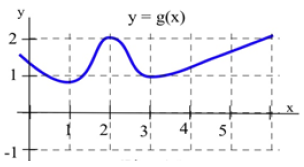
8.
(a) At what values of [latex]x[/latex] does the graph of [latex]f[/latex] in Fig. 41 have a horizontal tangent line?
(b) At what value(s) of [latex]x[/latex] is the value of [latex]f[/latex] the largest? Smallest?
(c) Sketch the graph of [latex]m(x)[/latex]= the slope of the line tangent to the graph of f at the point [latex](x,y)[/latex].
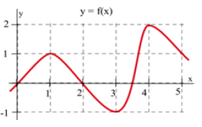
9.
(a) At what values of [latex]x[/latex] does the graph of [latex]g[/latex] in Fig. 42 have a horizontal tangent line?
(b) At what value(s) of [latex]x[/latex] is the value of [latex]g[/latex] the largest? Smallest?
(c) At what value(s) of [latex]x[/latex] is the slope of [latex]g[/latex] the largest? Smallest?
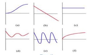
10.
Match the situation descriptions with the corresponding time–velocity graphs in Fig. 43.
(a) A car quickly leaving from a stop sign.
(b) A car sedately leaving from a stop sign.
(c) A student bouncing on a trampoline.
(d) A ball thrown straight up.
(e) A student confidently striding across campus to take a calculus test.
(f) An unprepared student walking across campus to take a calculus test.
11.
Fig. 44 shows the temperature during a summer day in Chicago. Sketch the graph of the rate at which the temperature is changing. (This is just the graph of the slopes of the lines that are tangent to the temperature graph.)
12.
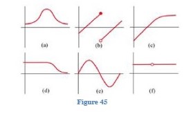
Fig. 45 shows six graphs, three of which are derivatives of the other three. Match the functions with their derivatives.
13.
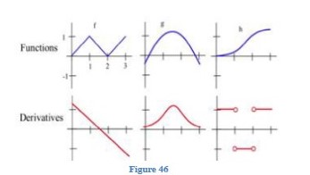
Match the graphs of the three functions in Fig. 46 with the graphs of their derivatives.
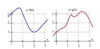
14. Use the information in Fig. 47 to plot the values of the functions [latex]f + g, \ f.g[/latex] and [latex]f/g[/latex] and their derivatives at [latex]x = 1[/latex], [latex]2[/latex], and [latex]3[/latex].
15.
Calculate [latex]\frac{d}{dx} \bigg( (x-5)(3x+1) \bigg)[/latex] by (a) using the product rule and (b) expanding the product and then differentiating. Verify that both methods give the same result.
16.
If the product of [latex]f[/latex] and [latex]g[/latex] is a constant ([latex]f(x) ∙ g(x) = k[/latex] for all [latex]x[/latex]), then how are [latex]\frac{\frac{d}{dx}\bigg( f(x) \bigg)}{f(x)}[/latex] and [latex]\frac{\frac{d}{dx}\bigg( g(x) \bigg)}{g(x)}[/latex] related?
17.
If the quotient of [latex]f[/latex] and [latex]g[/latex] is a constant (for all [latex]x[/latex]), then how are [latex]g . f '[/latex] and [latex]f . g '[/latex] related?
In problems 20–25, (a) calculate [latex]f '(1)[/latex] and (b) determine when [latex]f '(x) = 0[/latex].
18.
[latex]f(x) = x^2 – 5x + 13[/latex]
19.
[latex]f(x) = 5x^2 – 40x + 73[/latex]
20.
[latex]f(x) = x^3 + 9x^2 + 6[/latex]
21.
[latex]f(x) = x^3 + 3x^2 + 3x – 1[/latex]
22.
[latex]f(x) = x^3 + 2x^2 + 2x – 1[/latex]
23.
[latex]f(x) = \frac{7x}{x^2+4}[/latex]
24.
Determine [latex]\frac{d}{dx}\bigg( (x^2+1)(7x-3) \bigg)[/latex] and [latex]\frac{d}{dt} \bigg( \frac{3t-2}{5t+1} \bigg)[/latex].
25.
Find (a) [latex]\frac{d}{dx} \bigg( x^3e^x \bigg)[/latex] and (b) [latex]\frac{d}{dx} \bigg( e^x \bigg)^3[/latex].
26.
Find (a) [latex]\frac{d}{dt} \bigg( te^t \bigg)[/latex] and (b) [latex]\frac{d}{dx} \bigg( e^x \bigg)^3[/latex].
27:
Where do [latex]f(x) = x^2 – 10x + 3[/latex] and [latex]g(x) = x^3 – 12x[/latex] have horizontal tangent lines?
Brief Answers to Selected Exercises
1.
[latex]m = \frac{y-9}{x-3}[/latex]. If [latex]x = 2.97[/latex], then [latex]m = \frac{-0.1791-9}{-0.03} = 5.97[/latex]. If [latex]x = 3.001[/latex], then [latex]m = \frac{0.00601}{0.001} = 6.001[/latex].
If [latex]x = 3+h[/latex], then [latex]m = \frac{(3+h)^2-9}{((3+h)-3} = \frac{9+6h+h^2-9}{h} = 6+h[/latex]. When [latex]h[/latex] is very small (close to [latex]0[/latex]), [latex]6 + h[/latex] is very close to [latex]6[/latex].
3.
All of these answers are approximate. Your answers should be close to these numbers.
- [latex]\text{change} \approx \frac{80^o-64^o}{1 \text{pm} - 9 \text{am}} = \frac{16^o}{4 \text{hours}} = 4^o \text{per hour}[/latex].
- Use the slope of the tangent line. At [latex]10\ \text{am}[/latex], temperature was rising about [latex]5^{o}\ \text{per hour}[/latex]. At [latex]7 \text{pm}[/latex], temperature was rising about [latex]-10^{o}\ \text{per hour}[/latex] (falling about [latex]-10^{o}\ \text{per hour}[/latex]).
5.
All of these answers are approximate. Your answers should be close to these numbers.
- [latex]\text{average velocity} \approx \frac{300 \ \text{ft} - 0 \ \text{ft}}{20 \ \text{sec} - 0 \ \text{sec}}= -1\ \text{ feet per hour}[/latex].
- [latex]\text{average velocity} \approx \frac{100 \ \text{ft} - 200 \ \text{ft}}{30 \ \text{sec} - 20 \ \text{sec}}= - 5\ \text{ feet per hour}[/latex].
- At [latex]t = 10[/latex] seconds, [latex]\text{velocity} \approx 30 \ \text{ feet per second}[/latex] (between [latex]20[/latex] and [latex]35 \ \text{ft/s}[/latex]). At [latex]t = -1[/latex] seconds, [latex]\text{velocity} \approx 30\ \text{ feet per second}[/latex]. At [latex]t = 30[/latex] seconds, [latex]\text{velocity} \approx -40\ \text{ feet per second}[/latex].
7.
Fig. 1 is a graph of [latex]m(x)[/latex]. Approximate values of [latex]m(x)[/latex] are in the table.
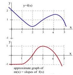
| x | y= f(x) | m(x) = the estimated slope of tangent line to y= f(x) at the point (x,y) |
|---|---|---|
| 0 | 2 | -1 |
| 1 | 1 | -1 |
| 2 | 1/3 | 0 |
| 3 | 1 | 1 |
| 4 | 3/2 | 1/2 |
| 5 | 1 | -2 |
9.
a. The graph of [latex]g[/latex] has a horizontal tangent line at about [latex]x = 1, x = 2[/latex], and [latex]x = 3[/latex].
b. [latex]g[/latex] is largest when [latex]x = 2[/latex] and for [latex]x = -0.5[/latex] and [latex]x = 6[/latex] (the edges of the graph). [latex]g[/latex] is smallest when [latex]x = 1[/latex] and [latex]x = 3[/latex].
c. The slope of [latex]g[/latex] is the largest when [latex]x = \ \text{about} \ 1.5[/latex], when the graph of [latex]g[/latex] is steepest while increasing. The slope of [latex]g[/latex] is smallest when [latex]x = \ \text{about} \ 2.5[/latex], when the graph of [latex]g[/latex] is steepest while decreasing.
11.
Fig. 2 is a graph of the approximate rate of temperature change (slope).
13.
The left derivative graph is [latex]g’[/latex]. The middle derivative graph is [latex]h'[/latex]. The right derivative graph is [latex]f’[/latex].
15.
a. [latex]\frac{d}{dx} \bigg( (x-5)(3x+7) \bigg) = (1)(3x+7)+(x-5)(3)=6x-8[/latex]
b. [latex]\frac{d}{dx} \bigg( (x-5)(3x+7) \bigg) =\frac{d}{dx} (3x^2-8x-35)=6x-8[/latex]
17.
If [latex]\frac{f(x)}{g(x)}= k[/latex], then [latex]\frac{d}{dx}\bigg( \frac{f(x)}{g(x)} \bigg) =0[/latex]. So the numerator of the rational function we’d get from the quotient rule must be zero; that is, [latex]f'g-fg' = 0[/latex]. So [latex]f'g[/latex] and [latex]fg'[/latex] are equal. (Another way to think about this: If [latex]\frac{f(x)}{g(x)}= k[/latex], then [latex]f(x)=kg(x)[/latex] and [latex]f'(x) = kg'g = kgg' = fg'[/latex].)
19.
If [latex]f(x) = x^2-5x+13[/latex], so [latex]f'(x) = 2x-5, \ f'(1) = 2-5=-3[/latex], and [latex]f'(x) = 2x-5 =0[/latex] when [latex]x=2.5[/latex].
21.
[latex]f(x) = x^3+3x^2+3x-1[/latex], so [latex]f'(x) = 3x^2+6x+3, f'(1) = 12[/latex], and [latex]f'(x) = 0[/latex] when [latex]x=-1[/latex].
23.
[latex]f(x) = \frac{7x}{x^2+4}[/latex], so [latex]f'(x) = \frac{(70)(x^2-4)-(7x)(2x)}{(x^2+4)^2} = \frac{-7x+28}{(x^2+4)^2}, f'(1) = \frac{21}{25}[/latex], and [latex]f(x) =0[/latex] when [latex]x=4[/latex].
25.
a. [latex]\frac{d}{dx}(x^3e^x)= (3x^2)(e^x) + (x^3)(e^x)[/latex].
b. [latex]\frac{d}{dx}(e^x)^3) = 3(e^x)^2(e^x) = 3e^{3x}[/latex].
Alternatively, [latex]\frac{d}{dx}(e^x)^3) = \frac{d}{dx}(e^{3x}) = 3e^{3x}[/latex].
