Chapter 3: Applications of the Derivative
Section 3.3: Applied Optimization
Learning Objectives
By the end of this section, the student should be able to:
- Solve minimum-maximum problems using calculus.
We have used derivatives to help find the maximums and minimums of some functions given by equations, but it is very unlikely that someone will simply hand you a function and ask you to find its extreme values. More typically, someone will describe a problem and ask your help in maximizing or minimizing something: What is the largest volume package which the post office will take?
; What is the quickest way to get from here to there?
; or What is the least expensive way to accomplish some task?
In this section, we’ll discuss how to find these extreme values using calculus.
Max/Min Applications
Example
The manager of a garden store wants to build a [latex]600[/latex]-square-foot rectangular enclosure on the store’s parking lot in order to display some equipment. Three sides of the enclosure will be built of redwood fencing, at a cost of [latex]\$7[/latex] per running foot. The fourth side will be built of cement blocks, at a cost of [latex]\$14[/latex] per running foot. Find the dimensions of the least costly enclosure.
The process of finding maxima or minima is called optimization. The function we’re optimizing is called the objective function (or objective equation). The objective function can be recognized by its proximity to est
words (e.g., greatest, least, highest, farthest). Look at the garden store example; the cost function is the objective function.
In many cases, there are two (or more) variables in the problem. In the garden store example again, the length and width of the enclosure are both unknown. If there is an equation that relates the variables, we can solve for one of them in terms of the others and write the objective function as a function of just one variable. Equations that relate the variables in this way are called constraint equations. The constraint equations are always equations, so they will have equals signs. For the garden store, the fixed area relates the length and width of the enclosure. This will give us our constraint equation.
Max-Min Story Problem Technique
- Translate the English statement of the problem line by line into a picture (if that applies) and into math. This is often the hardest step!
- Identify the objective function. Look for words indicating a largest or smallest value.
- If you seem to have two or more variables, find the constraint equation. Think about the English meaning of the word
constraint
and remember that the constraint equation will have an equals sign. - Solve the constraint equation for one variable and substitute into the objective function. Now you have an equation of one variable.
- If you seem to have two or more variables, find the constraint equation. Think about the English meaning of the word
- Use calculus to find the optimum values. (Take derivative, find critical points, test. Don’t forget to check the endpoints!)
- Look back at the question to make sure you answered what was asked. Translate your number answer back into English.
Here is a link to the examples used in the videos in this section: Applied Optimization Problems PDF.
Video
Example 1
The manager of a garden store wants to build a [latex]600[/latex]-square-foot rectangular enclosure on the store’s parking lot in order to display some equipment. Three sides of the enclosure will be built of redwood fencing, at a cost of [latex]$7[/latex] per running foot. The fourth side will be built of cement blocks, at a cost of [latex]$14[/latex] per running foot. Find the dimensions of the least costly enclosure.
First, translate line by line into math and a picture:
| Text | Translation |
| The manager of a garden store wants to build a [latex]600[/latex]-square-foot rectangular enclosure on the store’s parking lot in order to display some equipment.
Three sides of the enclosure will be built of redwood fencing, at a cost of $7 per running foot. The fourth side will be built of cement blocks, at a cost of $14 per running foot. Find the dimensions of the least costly such enclosure. |
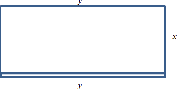
Let [latex]x[/latex] and [latex]y[/latex] be the dimensions of the enclosure, with [latex]y[/latex] being the length of the side made of blocks. Then: [latex]\text{Area} = A = xy = 600.[/latex]
[latex]2x + y[/latex] costs $7 per foot, [latex]y[/latex] costs $14 per foot, so [latex]\text{Cost} = C = 7(2x + y) + 14y = 14x + 21y.[/latex] Find [latex]x[/latex] and [latex]y[/latex] so that [latex]C[/latex] is minimized. |
The objective function is the cost function, and we want to minimize it. As it stands, though, it has two variables, so we need to use the constraint equation. The constraint equation is the fixed area [latex]A = xy = 600[/latex]. Solve [latex]A[/latex] for [latex]x[/latex] to get [latex]x=\frac{600}{y}[/latex], and then substitute into [latex]C[/latex]: [latex]C=14\left(\frac{600}{y}\right)+21y=\frac{8400}{y}+21y.[/latex]
Now we have a function of just one variable, so we can find the minimum using calculus:
[latex]C'=-\frac{8400}{y^2}+21[/latex] [latex]C'[/latex] is undefined for [latex]y = 0[/latex], and [latex]C' = 0[/latex] when [latex]y = 20[/latex] or [latex]y = -20[/latex].
Of these three critical numbers, only [latex]y = 20[/latex] makes sense (is in the domain of the actual function) – remember that [latex]y[/latex] is a length, so it can’t be negative, and [latex]y = 0[/latex] would mean there was no enclosure at all, so it couldn’t have an area of 600 square feet.
Test [latex]y = 20[/latex] (here we chose the second derivative test): [latex]C''=\frac{16800}{y^3} \gt 0,[/latex] so this is a local minimum.
Since this is the only critical point in the domain, this must be the global minimum. Going back to our constraint function, we can find that when [latex]y = 20[/latex], [latex]x = 30[/latex]. The dimensions of the enclosure that minimize the cost are 20 feet by 30 feet.
Video
When trying to maximize their revenue, businesses also face the constraint of consumer demand. While a business would love to see lots of products at a very high price, typically demand decreases as the price of goods increases. In simple cases, we can construct that demand curve to allow us to maximize revenue.
Example 2
A concert promoter has found that if she sells tickets for [latex]$50[/latex] each, she can sell [latex]1200[/latex] tickets, but for each [latex]$5[/latex] she raises the price, [latex]50[/latex] less people attend. What price should she sell the tickets at to maximize her revenue?
We are trying to maximize revenue, and we know that [latex]R=pq[/latex], where [latex]p[/latex] is the price per ticket and [latex]q[/latex] is the quantity of tickets sold.
The problem provides information about the demand relationship between price and quantity: as price increases, demand decreases. We need to find a formula for this relationship. To investigate, let’s calculate what will happen to attendance if we raise the price.
| Price, [latex]p[/latex] | [latex]50[/latex] | [latex]55[/latex] | [latex]60[/latex] | [latex]65[/latex] |
| Quantity, [latex]q[/latex] | [latex]1200[/latex] | [latex]1150[/latex] | [latex]1100[/latex] | [latex]1050[/latex] |
You might recognize this as a linear relationship. We can find the slope for the relationship by using two points: [latex]m=\frac{1150-1200}{55-50}=\frac{-50}{5}=-10.[/latex]
You may notice that the second step in that calculation corresponds directly to the statement of the problem: the attendance drops 50 people for every $5 the price increases.
Using the point-slope form of the line, we can write the equation relating price and quantity: [latex]q-1200=-10(p-50).[/latex]
Simplifying to slope-intercept form gives the demand equation [latex]q=1700-10p.[/latex]
Substituting this into our revenue equation, we get an equation for revenue involving only one variable: [latex]R=pq=p(1700-10p)=1700p-10p^2.[/latex]
Now we can find the maximum of this function by finding critical numbers. [latex]R'=1700-20p[/latex], so [latex]R'=0[/latex] when [latex]p = 85[/latex].
Using the second derivative test, [latex]R''=-20 \lt 0[/latex] (for any value of [latex]p[/latex]), so the critical number is a local maximum. Since it is the only critical number, we can also conclude that it is the global maximum.
The promoter will be able to maximize revenue by charging [latex]$85[/latex] per ticket. At this price, she will sell [latex]q=1700-10(85)=850[/latex] tickets, generating [latex]$72,250[/latex] in revenue.
Video
Video
Chapter Opener: Maximizing Revenue
From Calculus, Volume 1, by Strang and Herman, OpenStax (Web), licensed under a CC BY-NC-SA 4.0 License.
Owners of a car rental company have determined that if they charge customers [latex]p[/latex] dollars per day to rent a car, where [latex]50\le p\le 200[/latex], the number of cars [latex]n[/latex] they rent per day can be modeled by the linear function [latex]n(p)=1000-5p[/latex]. If they charge [latex]$50[/latex] per day or less, they will rent all their cars. If they charge [latex]$200[/latex] per day or more, they will not rent any cars. Assuming the owners plan to charge customers between $50 per day and [latex]$200[/latex] per day to rent a car, how much should they charge to maximize their revenue?
Solution
Step 1: Let [latex]p[/latex] be the price charged per car per day and let [latex]n[/latex] be the number of cars rented per day. Let [latex]R[/latex] be the revenue per day.
Step 2: The problem is to maximize [latex]R[/latex].
Step 3: The revenue (per day) is equal to the number of cars rented per day times the price charged per car per day—that is, [latex]R=n×p[/latex].
Step 4: Since the number of cars rented per day is modeled by the linear function [latex]n(p)=1000-5p[/latex], the revenue [latex]R[/latex] can be represented by the function [latex]R(p)=n×p=(1000-5p)p=-5{p}^{2}+1000p[/latex].
Step 5: Since the owners plan to charge between [latex]\$50[/latex] per car per day and [latex]\$200[/latex] per car per day, the problem is to find the maximum revenue [latex]R(p)[/latex] for [latex]p[/latex] in the closed interval [latex]\left[50,200\right][/latex].
Step 6: Since [latex]R[/latex] is a continuous function over the closed, bounded interval [latex]\left[50,200\right][/latex], it has an absolute maximum (and an absolute minimum) in that interval. To find the maximum value, look for critical numbers. The derivative is [latex]{R}^{\prime }(p)=-10p+1000[/latex]. Therefore, the critical number is [latex]p=100[/latex]. When [latex]p=100[/latex], [latex]R(100)=\$50,000[/latex]. When [latex]p=50[/latex], [latex]R(p)=\$37,500[/latex]. When [latex]p=200[/latex], [latex]R(p)=\$0[/latex]. Therefore, the absolute maximum occurs at [latex]p=\$100[/latex]. The car rental company should charge [latex]\$100[/latex] per day per car to maximize revenue as shown in the following figure.
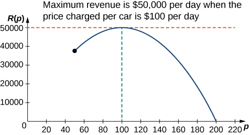
From Calculus, Volume 1, by Strang and Herman, OpenStax (Web), licensed under a CC BY-NC-SA 4.0 License.
A car rental company charges its customers [latex]p[/latex] dollars per day, where [latex]60\le p\le 150[/latex]. It has found that the number of cars rented per day can be modeled by the linear function [latex]n(p)=750-5p[/latex]. How much should the company charge each customer to maximize revenue?
Hint
[latex]R(p)=n×p[/latex], where [latex]n[/latex] is the number of cars rented and [latex]p[/latex] is the price charged per car.
Solution
The company should charge [latex]$75[/latex] per car per day.
Marginal Revenue = Marginal Cost
You may have heard before that profit is maximized when marginal cost and marginal revenue are equal.
Now you can see why people say that! (Even though it’s not completely true.)
Example 3
Suppose we want to maximize profit.
Now we know what to do – find the profit function, find its critical points, test them, etc.
But remember that profit = revenue – cost. So profit’ = revenue’ – cost’. That is, the derivative of the profit function is [latex]MR - MC[/latex].
Now let’s find the critical points – those will be where profit’ = 0 or is undefined. Profit’ = 0 when [latex]MR - MC = 0[/latex], or where [latex]MR = MC[/latex].
Key Takeaways
In all the cases we’ll see in this class, profit will be very well behaved, and we won’t have to worry about looking for critical points where profit is undefined. But remember that not all critical points are local max! The places where [latex]MR = MC[/latex] could represent local max, local min, or neither one.
Example 4
A company sells [latex]q[/latex] ribbon winders per year at [latex]\$p[/latex] per ribbon winder. The demand function for ribbon winders is given by [latex]p=300-0.02q[/latex]. The ribbon winders cost $30 apiece to manufacture, plus there are fixed costs of [latex]$9000[/latex] per year. Find the quantity where profit is maximized.
We want to maximize profit, but there isn’t a formula for profit given. So let’s make one. We can find a function for revenue = [latex]pq[/latex] using the demand function for [latex]p[/latex]. [latex]R(q)=(300-0.02q)q=300q-0.02q^2.[/latex]
We can also find a function for cost using the variable cost of [latex]$30[/latex] per ribbon winder, plus the fixed cost: [latex]C(q)=9000+30q.[/latex]
Putting them together, we get a function for profit: [latex]P(q)=R(q)-C(q)=\left(300q-0.02q^2\right)-(9000+30q)=-0.02q^2+270q-9000[/latex]
Now we have two choices. We can find the critical points of profit by taking the derivative of [latex]P(q)[/latex] directly, or we can find [latex]MR[/latex] and [latex]MC[/latex] and set them equal. (Naturally, we’ll get the same answer either way.)
Let’s use [latex]MR = MC[/latex] this time.
[latex]\begin{align*} MR=& 300-0.04q\\ MC=& 30\\ 300-0.04q=& 30\\ 270=& 0.04q\\ q=& 6750 \end{align*}[/latex]
The only critical point is at [latex]q = 6750[/latex]. Now we need to be sure this is a local max and not a local min. In this case, we’ll look to the graph of [latex]P(q)[/latex] – it’s a downward-opening parabola, so this must be a local max. And since it’s the only critical point, it must also be the global max.
Profit is maximized when they sell [latex]6750[/latex] ribbon winders.
Video
Average Cost = Marginal Cost
Average cost is minimized when average cost = marginal cost
is another saying that isn’t quite true; in this case, the correct statement is:
Key Takeaways
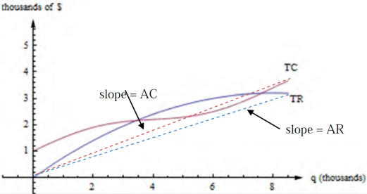
Let’s look at a geometric argument here. Remember that the average cost is the slope of the diagonal line, the line from the origin to the point on the total cost curve. If you move your clear plastic ruler around, you’ll see (and feel) that the slope of the diagonal line is smallest when the diagonal line just touches the cost curve – when the diagonal line is actually a tangent line – when the average cost is equal to the marginal cost.
Video
Media Attributions
- Triangle, Quality, Time image. © Pixabay is licensed under a CC0 (Creative Commons Zero) license
