Chapter 4: The Integral
Section 4.5: Average Value and the Net Change Theorem
Learning Objectives
By the end of this section, the student should be able to:
- Find the average value of a function.
- Explain the significance of the net change theorem.
- Use the net change theorem to solve applied problems.
Average Value
We know the average of [latex]n[/latex] numbers [latex]a_1, a_2, \dots , a_n[/latex] is their sum divided by [latex]n[/latex]. But what if we need to find the average temperature over a day’s time – there are too many possible temperatures to add them up! This is a job for the definite integral.
Video
Average Value
The average value of a function [latex]f(x)[/latex] on the interval [latex][a, b][/latex] is given by [latex]\frac{1}{b-a}\int_a^bf(x)\, dx[/latex].
Example 1
During a 9-hour work day, the production rate at time [latex]t[/latex] hours after the start of the shift was given by the function [latex]r(t)=5+\sqrt{t}[/latex] cars per hour. Find the average hourly production rate.
The average hourly production is [latex]\frac{1}{9-0}\int_0^9\left(5+\sqrt{t}\right)\, dt = 7[/latex] cars per hour.
A note about the units – remember that the definite integral has units (cars per hour) [latex]\cdot[/latex] (hours) = cars. But the [latex]\frac{1}{b-a}[/latex] in front has units [latex]\frac{1}{\text{hours}}[/latex] – the units of the average value are cars per hour, just what we expect an average rate to be.
Key Takeaways
In general…
…the average value of a function will have the same units as the integrand.
Function averages, involving means and more complicated averages, are used to smooth
data so that underlying patterns are more obvious and to remove high frequency noise
from signals. In these situations, the original function [latex]f[/latex] is replaced by some average of [latex]f[/latex].
If [latex]f[/latex] is rather jagged time data, then the 10-year average of [latex]f[/latex] is the integral [latex]g(x)=\frac{1}{10}\int\limits_{x-5}^{x+5} f(t)\, dt[/latex], an average of [latex]f[/latex] over 5 units on each side of [latex]x[/latex].
For example, the figure below shows the graphs of a monthly average (rather “noisy” data) of surface temperature data, an annual average (still rather jagged
), and a 5-year average (a much smoother function).

Typically, the average function reveals the pattern much more clearly than the original data. This use of a moving average
value of noisy
data (weather information, stock prices) is very common.
Video
Example 2
The graph below shows the amount of water in a reservoir over a 12-hour period. Estimate the average amount of water in the reservoir over this period.
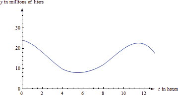
If [latex]V(t) [/latex] is the volume of the water (in millions of liters) after [latex]t[/latex] hours, then the average amount is [latex]\frac{1}{12}\,\int_0^{12} V(t)\, dt[/latex]. In order to find the definite integral, we’ll have to estimate. Let’s use 6 rectangles and take the heights from their right edges (there’s nothing special about using 6 rectangles or right edges – other choices would still give you a valid estimate).
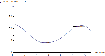
The estimate of the integral is [latex]\int_0^{12} V(t)\, dt \approx (18)(2)+(9.7)(2)+(8.2)(2)+(12)(2)+(19.9)(2)+(22)(2)=179.6.[/latex]
The units of this integral are (millions of liters) [latex]\cdot[/latex] (feet). So our estimate of the average volume is [latex]\frac{1}{12}\cdot 179.6\approx 15[/latex] millions of liters. (The estimate might change a little depending on how we estimate the function values from the graph.)
In the figure below, you can see the same graph with the line [latex]y=15[/latex] drawn in. The area under the curve and the area under the rectangle are (approximately) the same.
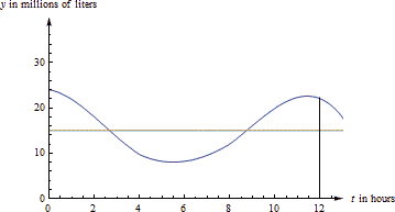
In fact, that would be a different way to estimate the average value. We could have estimated the placement of the horizontal line so that the area under the curve and under the line were equal.
The Net Change Theorem
[Content section from Calculus, Volume 1, by Strang and Herman, OpenStax (Web), licensed under a CC BY-NC-SA 4.0 License.]
The net change theorem considers the integral of a rate of change. It says that when a quantity changes, the new value equals the initial value plus the integral of the rate of change of that quantity. The formula can be expressed in two ways. The second is more familiar; it is simply the definite integral.
Net Change Theorem
The new value of a changing quantity equals the initial value plus the integral of the rate of change:
Subtracting [latex]F(a)[/latex] from both sides of the first equation yields the second equation. Since they are equivalent formulas, which one we use depends on the application.
The significance of the net change theorem lies in the results. Net change can be applied to area, distance, and volume, to name only a few applications. Net change accounts for negative quantities automatically without having to write more than one integral. To illustrate, let’s apply the net change theorem to a velocity function in which the result is displacement.
Suppose a car is moving due north (the positive direction) at 40 mph between 2 p.m. and 4 p.m., then the car moves south at 30 mph between 4 p.m. and 5 p.m. We can graph this motion as shown in Figure 1.
![A graph with the x axis marked as t and the y axis marked normally. The lines y=40 and y=-30 are drawn over [2,4] and [4,5], respectively.The areas between the lines and the x axis are shaded.](https://s3-us-west-2.amazonaws.com/courses-images/wp-content/uploads/sites/2332/2018/01/11204144/CNX_Calc_Figure_05_04_002.jpg)
Just as we did before, we can use definite integrals to calculate the net displacement as well as the total distance traveled. The net displacement is given by
Thus, at 5 p.m. the car is 50 miles north of its starting position. The total distance traveled is given by
Therefore, between 2 p.m. and 5 p.m., the car traveled a total of 110 miles.
To summarize, net displacement may include both positive and negative values. In other words, the velocity function accounts for both forward distance and backward distance. To find net displacement, integrate the velocity function over the interval. Total distance traveled, on the other hand, is always positive. To find the total distance traveled by an object, regardless of direction, we need to integrate the absolute value of the velocity function.
Finding the Net Displacement
Given a velocity function [latex]v(t)=3t-5[/latex] (in meters per second) for a particle in motion from time [latex]t=0[/latex] to time [latex]t=3[/latex], find the net displacement of the particle.
Solution
Applying the net change theorem, we have
The net displacement is [latex]-\frac{3}{2}[/latex] m. See Figure 2.
![A graph of the line v(t) = 3t – 5, which goes through points (0, -5) and (5/3, 0). The area over the line and under the x axis in the interval [0, 5/3] is shaded. The area under the line and above the x axis in the interval [5/3, 3] is shaded.](https://s3-us-west-2.amazonaws.com/courses-images/wp-content/uploads/sites/2332/2018/01/11204148/CNX_Calc_Figure_05_04_003.jpg)
Finding the Total Distance Traveled
Find the total distance traveled by a particle according to the velocity function [latex]v(t)=3t-5[/latex] m/sec over a time interval [latex]\left[0,3\right][/latex].
Solution
The total distance traveled includes both the positive and the negative values. Therefore, we must integrate the absolute value of the velocity function to find the total distance traveled.
To continue with the example, use two integrals to find the total distance. First, find the [latex]t[/latex]-intercept of the function, since that is where the division of the interval occurs. Set the equation equal to zero and solve for [latex]t[/latex]. Thus,
The two subintervals are [latex]\left[0,\frac{5}{3}\right][/latex] and [latex]\left[\frac{5}{3},3\right][/latex]. To find the total distance traveled, integrate the absolute value of the function. Since the function is negative over the interval [latex]\left[0,\frac{5}{3}\right][/latex], we have [latex]|v(t)|=-v(t)[/latex] over that interval. Over [latex]\left[\frac{5}{3},3\right][/latex], the function is positive, so [latex]|v(t)|=v(t)[/latex]. Thus, we have
So the total distance traveled is [latex]\frac{14}{6}[/latex] m.
Find the net displacement and total distance traveled in meters given the velocity function [latex]f(t)=\frac{1}{2}{e}^{t}-2[/latex] over the interval [latex]\left[0,2\right][/latex].
Solution
Net displacement: [latex]\frac{{e}^{2}-9}{2}\approx -0.8055\text{m;}[/latex] total distance traveled: [latex]4\text{ln}4-7.5+\frac{{e}^{2}}{2}\approx 1.740[/latex] m
Applying the Net Change Theorem
[Content section from Calculus, Volume 1, by Strang and Herman, OpenStax (Web), licensed under a CC BY-NC-SA 4.0 License.]
The net change theorem can be applied to the flow and consumption of fluids, as shown in the following example.
How Many Gallons of Gasoline Are Consumed?
If the motor on a motorboat is started at [latex]t=0[/latex] and the boat consumes gasoline at the rate of [latex]5-{t}^{3}[/latex] gal/hr, how much gasoline is used in the first 2 hours?
Solution
Express the problem as a definite integral, integrate, and evaluate using the fundamental theorem of calculus. The limits of integration are the endpoints of the interval [latex]\left[0,2\right][/latex]. We have
Thus, the motorboat uses 6 gal of gas in 2 hours.
Chapter Opener: Iceboats
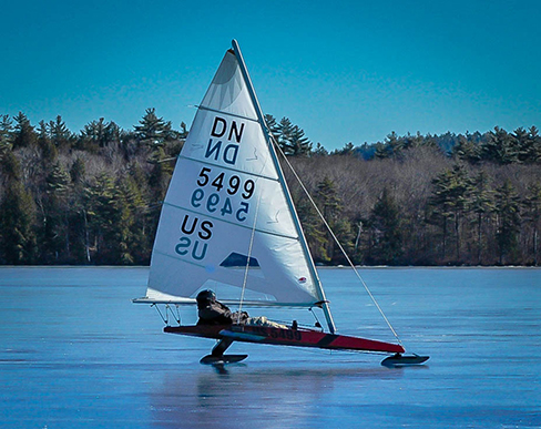
As we saw at the beginning of the chapter, top iceboat racers can attain speeds of up to five times the wind speed. Andrew is an intermediate iceboater, though, so he attains speeds equal to only twice the wind speed. Suppose Andrew takes his iceboat out one morning when a light 5-mph breeze has been blowing all morning. As Andrew gets his iceboat set up, though, the wind begins to pick up. During his first half hour of iceboating, the wind speed increases according to the function [latex]v(t)=20t+5[/latex]. For the second half hour of Andrew’s outing, the wind remains steady at 15 mph. In other words, the wind speed is given by
Recalling that Andrew’s iceboat travels at twice the wind speed, and assuming he moves in a straight line away from his starting point, how far is Andrew from his starting point after 1 hour?
Solution
To figure out how far Andrew has traveled, we need to integrate his velocity, which is twice the wind speed. Then
distance [latex]={\int }_{0}^{1}2v(t)dt[/latex].
Substituting the expressions we were given for [latex]v(t)[/latex], we get
Andrew is 25 miles from his starting point after 1 hour.
Suppose that instead of remaining steady during the second half hour of Andrew’s outing, the wind starts to die down according to the function [latex]v(t)=-10t+15[/latex]. In other words, the wind speed is given by
Under these conditions, how far from his starting point is Andrew after 1 hour?
Solution
17.5 miles
Hint
Don’t forget that Andrew’s iceboat moves twice as fast as the wind.
Media Attributions
- image054 © Robert A. Rohde is licensed under a CC BY (Attribution) license

Hint
Follow the procedures from the last two examples. Note that [latex]f(t)\le 0[/latex] for [latex]t\le \text{ln}4[/latex] and [latex]f(t)\ge 0[/latex] for [latex]t\ge \text{ln}4[/latex].