Chapter 2: Limits and The Derivative
Section 2.1: Limits and Continuity
Learning Objectives
By the end of this section, the student should be able to:
- Calculate the limit of a function using tables and graphs.
- Identify and give examples where a limit doesn’t exist for a function.
- Describe the relationship between one-sided limits, two-sided limits, and continuity.
- State the conditions for the continuity of a function.
Pre-calculus Idea: Slope and Rate of Change
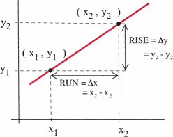
The slope of a line measures how fast a line rises or falls as we move from left to right along the line. It measures the rate of change of the y-coordinate with respect to changes in the x-coordinate. If the line represents the distance traveled over time, for example, then its slope represents the velocity. In the figure, you can remind yourself of how we calculate slope using two points on the line:
We would like to be able to get that same sort of information (how fast the curve rises or falls, velocity from distance) even if the graph is not a straight line. But what happens if we try to find the slope of a curve, as in the figure below?
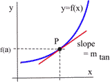
We need two points in order to determine the slope of a line. How can we find a slope of a curve, at just one point? The answer, as suggested in the figure, is to find the slope of the tangent line to the curve at that point. Most of us have an intuitive idea of what a tangent line is. Unfortunately, “tangent line” is hard to define precisely.
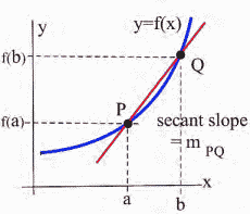
Definition (Secant Line)
A secant line is a line between two points on a curve.
See the image below:
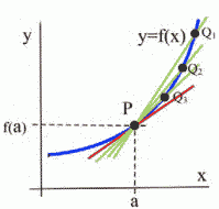
Can’t-Quite-Do-It-Yet Definition (Tangent Line)
A tangent line is a line at one point on a curve…that does its best to be the curve at that point?
As you may be able to see in the image below, the closer the point [latex]Q[/latex] is to the point [latex]P[/latex], the closer the secant slope gets to the tangent slope. This will be key to finding the tangent slope, but first, we need to more carefully define the idea of getting closer to.
Limits
In the last section, we saw that as the interval over which we calculated got smaller, the secant slopes approached the tangent slope. The limit gives us better language with which to discuss the idea of “approaches.”
The limit of a function describes the behavior of the function when the variable is near, but does not equal, a specified number (see the figure below).
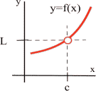
Definition (Limit)
If the values of [latex]f(x)[/latex] get closer and closer, as close as we want, to one number [latex]L[/latex] as we take values of [latex]x[/latex] very close to (but not equal to) a number [latex]c[/latex], then we say “the limit of [latex]f(x)[/latex] as [latex]x[/latex] approaches [latex]c[/latex] is [latex]L[/latex]” and we write [latex]\lim\limits_{x\to c} f(x)=L.[/latex] The symbol “[latex]\to[/latex]” means “approaches” or, less formally, “gets very close to”.
(This definition of the limit isn’t stated as formally as it could be, but it is sufficient for our purposes in this course.)
Note:
- [latex]f(c)[/latex] is a single number that describes the behavior (value) of [latex]f(x)[/latex] at the point [latex]x = c[/latex].
- [latex]\lim\limits_{x\to c} f(x)[/latex] is a single number that describes the behavior of [latex]f(x)[/latex] near, but not at, the point [latex]x = c[/latex].
If we have a graph of the function near x = c, then it is usually easy to determine [latex]\lim\limits_{x\to c} f(x)[/latex].
Video
Example 1
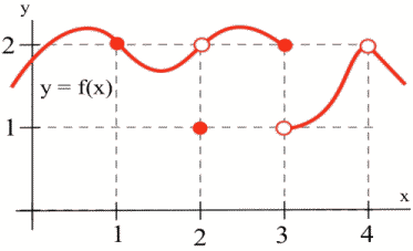
Use the graph of [latex]y = f(x)[/latex] in the figure below to determine the following limits:
- [latex]\lim\limits_{x\to 1} f(x)[/latex]
- [latex]\lim\limits_{x\to 2} f(x)[/latex]
- [latex]\lim\limits_{x\to 3} f(x)[/latex]
- [latex]\lim\limits_{x\to 4} f(x)[/latex]
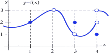
- When [latex]x[/latex] is very close to 1, the values of [latex]f(x)[/latex] are very close to [latex]y = 2[/latex]. In this example, it happens that [latex]f(1) = 2[/latex], but that is irrelevant for the limit. The only thing that matters is what happens for [latex]x[/latex] close to [latex]1[/latex] but [latex]x \neq 1[/latex].
- [latex]f(2)[/latex] is undefined, but we only care about the behavior of [latex]f(x)[/latex] for [latex]x[/latex] close to [latex]2[/latex] but not equal to [latex]2[/latex]. When [latex]x[/latex] is close to [latex]2[/latex], the values of [latex]f(x)[/latex] are close to [latex]3[/latex]. If we restrict [latex]x[/latex] close enough to [latex]2[/latex], the values of [latex]y[/latex] will be as close to [latex]3[/latex] as we want, so [latex]\lim\limits_{x\to 2} f(x) = 3[/latex].
- When [latex]x[/latex] is close to [latex]3[/latex] (or “as [latex]x[/latex] approaches the value 3″), the values of [latex]f(x)[/latex] are close to [latex]1[/latex] (or “approach the value [latex]1[/latex]“), so [latex]\lim\limits_{x\to 3} f(x) = 1[/latex]. For this limit it is completely irrelevant that [latex]f(3) = 2[/latex]. We only care about what happens to [latex]f(x)[/latex] for [latex]x[/latex] close to and not equal to [latex]3[/latex].
- This one is harder and we need to be careful. When [latex]x[/latex] is close to [latex]4[/latex] and slightly less than [latex]4[/latex] ([latex]x[/latex] is just to the left of [latex]4[/latex] on the [latex]x[/latex]-axis), then the values of [latex]f(x)[/latex] are close to [latex]2[/latex]. But if [latex]x[/latex] is close to [latex]4[/latex] and slightly larger than [latex]4[/latex], then the values of [latex]f(x)[/latex] are close to [latex]3[/latex]. If we only know that [latex]x[/latex] is very close to [latex]4[/latex], then we cannot say whether [latex]y = f(x)[/latex] will be close to [latex]2[/latex] or close to [latex]3[/latex]–it depends on whether [latex]x[/latex] is on the right or the left side of [latex]4[/latex]. In this situation, the [latex]f(x)[/latex] values are not close to a single number, so we say [latex]f(x)[/latex] does not exist. It is irrelevant that [latex]f(4) = 1[/latex]. The limit, as [latex]x[/latex] approaches [latex]4[/latex], would still be undefined if [latex]f(4)[/latex] was [latex]3[/latex] or [latex]2[/latex] or anything else.
We can also explore limits using tables and using algebra.
Video
Example 2
Find [latex]\lim\limits_{x\to 1} \dfrac{2x^2-x-1}{x-1}[/latex].
You might try to evaluate at [latex]x = 1[/latex], but [latex]f(x)[/latex] is not defined at [latex]x = 1[/latex]. It is tempting, but incorrect, to conclude that this function does not have a limit as [latex]x[/latex] approaches 1.
Using tables: Trying some “test” values for x that get closer and closer to 1 from both the left and the right, we get
| [latex]x[/latex] | [latex]f(x)[/latex] |
| [latex]0.9[/latex] | [latex]2.82[/latex] |
| [latex]0.9998[/latex] | [latex]2.9996[/latex] |
| [latex]0.999994[/latex] | [latex]2.999988[/latex] |
| [latex]0.9999999[/latex] | [latex]2.9999998[/latex] |
| [latex]\to 1[/latex] | [latex]\to 3[/latex] |
| [latex]x[/latex] | [latex]f(x)[/latex] |
| [latex]1.1[/latex] | [latex]3.2[/latex] |
| [latex]1.003[/latex] | [latex]3.006[/latex] |
| [latex]1.0001[/latex] | [latex]3.0002[/latex] |
| [latex]1.000007[/latex] | [latex]3.000014[/latex] |
| [latex]\to 1[/latex] | [latex]\to 3[/latex] |
The function [latex]f[/latex] is not defined at [latex]x = 1[/latex], but when [latex]x[/latex] is close to 1, the values of [latex]f(x)[/latex] are getting very close to 3. We can get [latex]f(x)[/latex] as close to 3 as we want by taking [latex]x[/latex] very close to 1 so [latex]\lim\limits_{x\to 1} \dfrac{2x^2-x-1}{x-1}=3.[/latex]
Using algebra: We could have found the same result by noting that [latex]f(x)= \dfrac{2x^2-x-1}{x-1} = \dfrac{(2x+1)(x-1)}{(x-1)} = 2x+1[/latex] as long as [latex]x \neq 1[/latex]. (If [latex]x\neq 1[/latex], then [latex]x–1 \neq 0[/latex], so it is valid to divide the numerator and denominator by the factor [latex]x–1[/latex].) The “[latex]x\to 1[/latex]” part of the limit means that x is close to 1 but not equal to 1, so our division step is valid and [latex]\lim\limits_{x\to 1}\dfrac{2x^2-x-1}{x-1} = \lim\limits_{x\to 1} 2x+1 = 3,[/latex] which is our answer.
Using a graph: We can graph [latex]y=f(x)= \dfrac{2x^2-x-1}{x-1}[/latex] for [latex]x[/latex] close to 1:
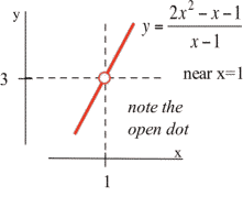
Notice that whenever [latex]x[/latex] is close to 1, the values of [latex]y = f(x)[/latex] are close to 3. Since [latex]f[/latex] is not defined at [latex]x = 1[/latex], the graph has a hole above [latex]x = 1[/latex], but we only care about what [latex]f(x)[/latex] is doing for [latex]x[/latex] close to but not equal to 1.
Video
One Sided Limits
Sometimes, what happens to us at a place depends on the direction we use to approach that place. If we approach Niagara Falls from the upstream side, then we will be 182 feet higher and have different worries than if we approach from the downstream side. Similarly, the values of a function near a point may depend on the direction we use to approach that point.
Definition (Left and Right Limits)
The left limit of [latex]f(x)[/latex] as [latex]x[/latex] approaches [latex]c[/latex] is [latex]L[/latex] if the values of [latex]f(x)[/latex] get as close to [latex]L[/latex] as we want when [latex]x[/latex] is very close to and left of [latex]c[/latex] (i.e., [latex]x \lt c[/latex]). We write [latex]\lim\limits_{x\to c^-} f(x)=L.[/latex]
The right limit of [latex]f(x)[/latex] as [latex]x[/latex] approaches [latex]c[/latex] is [latex]L[/latex] if the values of [latex]f(x)[/latex] get as close to [latex]L[/latex] as we want when [latex]x[/latex] is very close to and right of [latex]c[/latex] (i.e., [latex]x \gt c[/latex]). We write [latex]\lim\limits_{x\to c^+} f(x)=L.[/latex]
Example 3
Evaluate the one sided limits of the function [latex]f(x)[/latex] graphed below at [latex]x = 0[/latex] and [latex]x = 1[/latex].
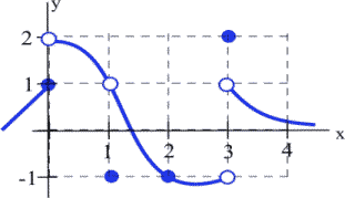
As [latex]x[/latex] approaches 0 from the left, the value of the function is getting closer to 1, so [latex]\lim\limits_{x\to 0^-} f(x) = 1[/latex].
As [latex]x[/latex] approaches 0 from the right, the value of the function is getting closer to 2, so [latex]\lim\limits_{x\to 0^+} f(x) = 2[/latex].
Notice that since the limit from the left and limit from the right are different, the general limit, [latex]\lim\limits_{x\to 0} f(x)[/latex], does not exist.
At [latex]x[/latex] approaches 1 from either direction, the value of the function is approaching 1, so [latex]\lim\limits_{x\to 1^-} f(x) = \lim\limits_{x\to 1^+} f(x) = \lim\limits_{x\to 1} f(x) = 1.[/latex]
Video
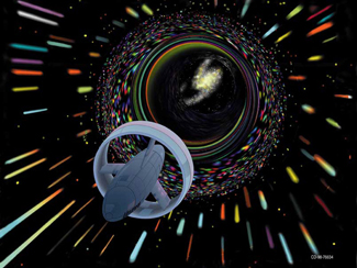
Chapter Opener: Einstein’s Equation
From Calculus, Volume 1, by Strang and Herman, OpenStax (Web), licensed under a CC BY-NC-SA 4.0 License.
In the chapter opener, we mentioned briefly how Albert Einstein showed that a limit exists to how fast any object can travel. Given Einstein’s equation for the mass of a moving object, what is the value of this bound?
Solution
Our starting point is Einstein’s equation for the mass of a moving object,
where [latex]m_0[/latex] is the object’s mass at rest, [latex]v[/latex] is its speed, and [latex]c[/latex] is the speed of light. To see how the mass changes at high speeds, we can graph the ratio of masses [latex]m/m_0[/latex] as a function of the ratio of speeds, [latex]v/c[/latex] ( Figure 12).
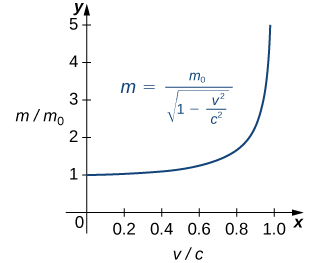
We can see that as the ratio of speeds approaches 1—that is, as the speed of the object approaches the speed of light—the ratio of masses increases without bound. In other words, the function has a vertical asymptote at [latex]v/c=1[/latex]. We can try a few values of this ratio to test this idea.
| [latex]\frac{v}{c}[/latex] | [latex]\sqrt{1-\frac{v^2}{c^2}}[/latex] | [latex]\frac{m}{m_0}[/latex] |
|---|---|---|
| 0.99 | 0.1411 | 7.089 |
| 0.999 | 0.0447 | 22.37 |
| 0.9999 | 0.0141 | 70.71 |
Thus, if an object with mass 100 kg is traveling at 0.9999[latex]c[/latex], its mass becomes 7071 kg. Since no object can have an infinite mass, we conclude that no object can travel at or more than the speed of light.
Continuity
A function that is “friendly” and doesn’t have any breaks or jumps in it is called continuous. More formally,
Definition (Continuity at a Point)
A function [latex]f(x)[/latex] is continuous at [latex]x = a[/latex] if and only if [latex]\lim\limits_{x\to a} f(x) = f(a)[/latex].
The graph below illustrates some of the different ways a function can behave at and near a point, and the table contains some numerical information about the function and its behavior.
| [latex]a[/latex] | [latex]f(a)[/latex] | [latex]\lim\limits_{x\to a} f(x)[/latex] |
| [latex]1[/latex] | [latex]2[/latex] | [latex]2[/latex] |
| [latex]2[/latex] | [latex]1[/latex] | [latex]2[/latex] |
| [latex]3[/latex] | [latex]2[/latex] | Does not exist (DNE) |
| [latex]4[/latex] | Undefined | [latex]2[/latex] |
Based on the information in the table, we can conclude that [latex]f[/latex] is continuous at 1, since [latex]\lim\limits_{x\to 1} f(x) = 2 = f(1)[/latex]. We can also conclude from the information in the table that [latex]f[/latex] is not continuous at 2 or 3 or 4, because [latex]\lim\limits_{x\to 2} f(x) \neq f(2)[/latex], [latex]\lim\limits_{x\to 3} f(x) \neq f(3)[/latex], and [latex]\lim\limits_{x\to 4} f(x) \neq f(4)[/latex].
The behaviors at [latex]x = 2[/latex] and [latex]x = 4[/latex] exhibit a hole in the graph, sometimes called a removable discontinuity, since the graph could be made continuous by changing the value of a single point. The behavior at [latex]x = 3[/latex] is called a jump discontinuity, since the graph jumps between two values. Jump discontinuities and vertical asymptotes are both nonremovable discontinuities because they cannot be fixed by changing the value of a single point.
So which functions are continuous? It turns out that pretty much every function you’ve studied is continuous where it is defined: polynomial, radical, rational, exponential, and logarithmic functions are all continuous where they are defined. Moreover, any combination of continuous functions is also continuous.
This is helpful because the definition of continuity says that for a continuous function, [latex]\lim\limits_{x\to a} f(x) = f(a)[/latex]. That means for a continuous function, we can find the limit by direct substitution (evaluating the function) if the function is continuous at [latex]a[/latex].
Video
Example 4
Evaluate using continuity, if possible:
- [latex]\lim\limits_{x\to 2} x^3-4x[/latex]
- [latex]\lim\limits_{x\to 2} \dfrac{x-4}{x+3}[/latex]
- [latex]\lim\limits_{x\to 2} \dfrac{x-4}{x-2}[/latex]
- The given function is polynomial and is defined for all values of x, so we can find the limit by direct substitution: [latex]\lim\limits_{x\to 2} x^3-4x = 2^3-4(2) = 0.[/latex]
- The given function is rational. It is not defined at x = -3, but we are taking the limit as x approaches 2, and the function is defined at that point, so we can use direct substitution: [latex]\lim\limits_{x\to 2} \dfrac{x-4}{x+3} = \dfrac{2-4}{2+3}= -\dfrac{2}{5}.[/latex]
- This function is not defined at x = 2, and so is not continuous at x = 2. We cannot use direct substitution.
Media Attributions
- image002
- image111
- image112
- image011
- image012
- image013
- image014
- CNX_Calc_Figure_02_02_017
- image015
change in the vertical coordinates (rise) to the change in the horizontal coordinates (run) between two points on a line. m = difference in y coordinates divided by the difference in x coordinates.
