Chapter 4: The Integral
Section 4.6: Applications to Business
Learning Objectives
By the end of this section, the student should be able to:
- Solve consumer and producer surplus problems.
- Solve continuous income stream problems.
Consumer and Producer Surplus
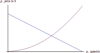
Here is a demand and supply curve for a product. Which is which?

The demand curve is decreasing. Lower prices are associated with higher quantities demanded; higher prices are associated with lower quantities demanded. Demand curves are often shown as if they were linear, but there’s no reason they have to be.
The supply curve is increasing. Lower prices are associated with lower supply, and higher prices are associated with higher quantities supplied.
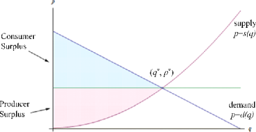
The point where the demand and supply curves cross is called the equilibrium point [latex](q^*, p^*)[/latex].

Suppose that the price is set at the equilibrium price so that the quantity demanded equals the quantity supplied. Now think about the folks who are represented on the left of the equilibrium point. The consumers on the left would have been willing to pay a higher price than they ended up having to pay, so the equilibrium price saved them money. On the other hand, the producers represented on the left would have been willing to supply these goods for a lower price – they made more money than they expected to. Both of these groups ended up with extra cash in their pockets!
Graphically, the amount of extra money that ended up in consumers' pockets is the area between the demand curve and the horizontal line at [latex]p^*[/latex]. This is the difference in price, summed up over all the consumers who spent less than they expected to – a definite integral. Notice that since the area under the horizontal line is a rectangle, we can simplify the area integral: [latex]\int\limits_0^{q^*} \left( d(q)-p^*\right)\, dq = \int\limits_0^{q^*} d(q)\, dq – \int\limits_0^{q^*} p^*\, dq = \int\limits_0^{q^*} d(q)\, dq – p^*q^*.[/latex]
The amount of extra money that ended up in producers' pockets is the area between the supply curve and the horizontal line at [latex]p^*[/latex]. This is the difference in price, summed up over all the producers who received more than they expected to. Similar to consumer surplus, this integral can be simplified: [latex]\int\limits_0^{q^*} \left( p^*-s(q) \right)\, dq = \int\limits_0^{q^*} p^*\, dq - \int\limits_0^{q^*} s(q)\, dq = p^*q^* - \int\limits_0^{q^*} s(q)\, dq.[/latex]
Consumer and Producer Surplus
Given a demand function [latex]p = d(q)[/latex] and a supply function [latex]p = s(q)[/latex], and the equilibrium point [latex](q^*, p^*)[/latex]:
- The consumer surplus is [latex]\int\limits_0^{q^*} d(q)\, dq – p^*q^*.[/latex]
- The producer surplus is [latex]p^*q^* - \int\limits_0^{q^*} s(q)\, dq.[/latex]
- The sum of the consumer surplus and producer surplus is the total gains from trade.
What are the units of consumer and producer surplus? The units are (price per item)(quantity of items) = money!
Video
Example 1
Suppose the demand for a product is given by [latex]p=d(q)=-0.8q+150[/latex] and the supply for the same product is given by [latex]p=s(q)=5.2q[/latex]. For both functions, [latex]q[/latex] is the quantity and [latex]p[/latex] is the price, in dollars.
- Find the equilibrium point.
- Find the consumer surplus at the equilibrium price.
- Find the producer surplus at the equilibrium price.
- The equilibrium point is where the supply and demand functions are equal. Solving [latex]-0.8q+150 = 5.2q[/latex] gives [latex]q = 25[/latex].
- The consumer surplus is [latex]\int\limits_0^{25} (-0.8q+150)\, dq – (130)(25) = \$ 250.[/latex]
- The producer surplus is [latex](130)(25) - \int\limits_0^{25} 5.2q\, dq = \$ 1625.[/latex]
Example 2
The tables below show information about the demand and supply functions for a product. For both functions, [latex]q[/latex] is the quantity and [latex]p[/latex] is the price, in dollars.
| q | 0 | 100 | 200 | 300 | 400 | 500 | 600 | 700 |
| p | 70 | 61 | 53 | 46 | 40 | 35 | 31 | 28 |
| q | 0 | 100 | 200 | 300 | 400 | 500 | 600 | 700 |
| p | 14 | 21 | 28 | 33 | 40 | 47 | 54 | 61 |
- Which is which? That is, which table represents demand and which represents supply?
- What is the equilibrium price and quantity?
- Find the consumer and producer surplus at the equilibrium price.
Answers:
- The first table shows decreasing price associated with increasing quantity, so that is the demand function. The second table shows increasing price associated with increasing quantity, so that is the supply function.
- For both functions, [latex]q = 400[/latex] is associated with [latex]p = 40[/latex]; the equilibrium price is $40 and the equilibrium quantity is 400 units. Notice that we were lucky here, because the equilibrium point is actually one of the points shown. In many cases with a table, we would have to estimate.
- The consumer surplus uses the demand function, which comes from the first table. We'll have to approximate the value of the integral using rectangles. There are 4 rectangles, and let's choose to use left endpoints. The consumer surplus is
[latex]\begin{align*} \int\limits_0^{400} \text{(demand)}\, dq-(40)(400)\approx & \\ (100)(70+61+53+46)-(40)(400)=& \$7000 \end{align*}[/latex]
So the consumer surplus is about $7000. The producer surplus uses the supply function, which comes from the second table. Let's choose to use left endpoints for this integral also. The producer surplus is
[latex]\begin{align*} (40)(400)-\int\limits_0^{400} \text{(supply)}\, dq \approx & \\ (40)(400)-(100)(14+21+28+33)=& \$6400 \end{align*}[/latex]
So the producer surplus is about $6400.
Continuous Income Stream
In precalculus, you learned about compound interest in that really simple situation where you made a single deposit into an interest-bearing account and let it sit undisturbed, earning interest, for some period of time.
Recall:
Compound Interest Formulas
Let [latex]P[/latex] be the principal (initial investment), [latex]r[/latex] be the annual interest rate expressed as a decimal, and [latex]A(t)[/latex] be the amount in the account at the end of [latex]t[/latex] years.
Compounding [latex]n[/latex] Times per Year
[latex]A(t) = P\left(1+\frac{r}{n}\right)^{nt}[/latex]
Compounded Continuously
[latex]A(t)=Pe^{rt}[/latex]
If you’re using this formula to find what an account will be worth in the future, [latex]t \gt 0[/latex] and [latex]A(t)[/latex] is called the future value.
If you're using the formula to find what you need to deposit today to have a certain value [latex]P[/latex] sometime in the future, [latex]t \lt 0[/latex] and [latex]A(t)[/latex] is called the present value.
You may also have learned somewhat more complicated annuity formulas to deal with slightly more complicated situations – where you make equal deposits equally spaced in time.
But real life is not usually so neat.
Calculus allows us to handle situations where deposits
are flowing continuously into an account that earns interest. As long as we can model the flow of income with a function, we can use a definite integral to calculate the present and future value of a continuous income stream. The idea here is that each little bit of income in the future needs to be multiplied by the exponential function to bring it back to the present, and then we'll add them all up (a definite integral).
Continuous Income Stream
Suppose money can earn interest at an annual interest rate of r, compounded continuously. Let [latex]F(t)[/latex] be a continuous income function (in dollars per year) that applies between year [latex]0[/latex] and year [latex]T[/latex].
Then the present value of that income stream is given by [latex]PV = \int\limits_0^T F(t)e^{-rt}\, dt.[/latex]
The future value can be computed by the ordinary compound interest formula [latex]FV = PVe^{rt}.[/latex]
This is a useful way to compare two investments – find the present value of each to see which is worth more today.
Video
Example 3
You have an opportunity to buy a business that will earn $75,000 per year continuously over the next eight years. Money can earn 2.8% per year, compounded continuously. Is this business worth its purchase price of $630,000?
First, please note that we still have to make some simplifying assumptions. We have to assume that the interest rates are going to remain constant for that entire eight years. We also have to assume that the $75,000 per year is coming in continuously, like a faucet dripping dollars into the business. Neither of these assumptions might be accurate.
But moving on: The present value of the $630,000 is, well, $630,000. This is one investment, where we put our $630,000 in the bank and let it sit there.
To find the present value of the business, we think of it as an income stream. The function [latex]F(t)[/latex] in this case is a constant $75,000 dollars per year, so [latex]F(t) = 75,\!000[/latex]. The interest rate is 2.8% and the term we're interested in is eight years, so [latex]r = .028[/latex], and [latex]T = 8:[/latex] [latex]PV=\int\limits_0^8 75000e^{-0.028t}\, dt \approx 537,\!548.75[/latex]
The present value of the business is about $537,500, which is less than the $630,000 asking price, so this is not a good deal.
While this integral could have been done using substitution, for many of the integrals in this section, we don't have the techniques to use antiderivatives or, in some cases, no antiderivative exists. Technology will work quickly, and it will give you an answer that is good enough.
Example 4
A company is considering purchasing a new machine for its production floor. The machine costs $65,000. The company estimates that the additional income from the machine will be a constant $7000 for the first year, then will increase by $800 each year after that. In order to buy the machine, the company needs to be convinced that it will pay for itself by the end of 8 years with this additional income. Money can earn 1.7% per year, compounded continuously. Should the company buy the machine?
We'll assume that the income will come in continuously over the 8 years. We’ll also assume that interest rates will remain constant over that 8-year time period.
We're interested in the present value of the machine, which we will compare to its $65,000 price tag. Let [latex]t[/latex] be the time, in years, since the purchase of the machine. The income from the machine is different depending on the time.
From [latex]t = 0[/latex] to [latex]t = 1[/latex] (the first year), the income is constant $7000 per year. From [latex]t = 1[/latex] to [latex]t = 8[/latex], the income is increasing by $800 each year; the income flow function [latex]F(t)[/latex] will be [latex]F(t)=7000+800(t-1)=6200+800t[/latex]. To find the present value, we'll have to divide the integral into the two pieces, one for each of the functions: [latex]PV=\int\limits_0^1 7000e^{-0.017t}\, dt + \int\limits_1^8 (6200+800t)e^{-0.017t}\, dt \approx 70166.[/latex]
The present value is greater than the cost of the machine, so the company should buy the machine.
Media Attributions
- image062
- image063

