Chapter 1 Linear Equations
1.3 Graph Linear Equations in Two Variables
Learning Objectives
By the end of this section, you will be able to:
- Plot points in a rectangular coordinate system
- Graph a linear equation by plotting points
- Graph vertical and horizontal lines
- Find the x- and y-intercepts
- Graph a line using the intercepts
Plot Points on a Rectangular Coordinate System
Just like maps use a grid system to identify locations, a grid system is used in mathematics to locate points in a plane. This grid system is called the rectangular coordinate system, or the Cartesian coordinate system, which is named after Rene’ Descartes, the French mathematician who is credited with developing this grid system in the seventeenth century.
The rectangular coordinate system is formed by two intersecting number lines, one horizontal and one vertical. The horizontal number line is called the x-axis. The vertical number line is called the y-axis. These axes divide a plane into four regions, called quadrants. The quadrants are identified by Roman numerals, beginning on the upper right and proceeding counterclockwise.
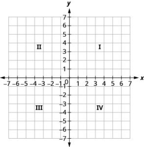
In the rectangular coordinate system, every point is represented by an ordered pair. The first number in the ordered pair is the x-coordinate of the point, and the second number is the y-coordinate of the point. The phrase “ordered pair” means that the order is important.
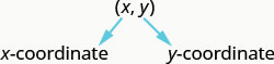
Ordered Pair
An ordered pair, [latex](x,y)[/latex] gives the coordinates of a point in a rectangular coordinate system. The first number is the x-coordinate. The second number is the y-coordinate.
What is the ordered pair of the point where the axes cross? At that point both coordinates are zero, so its ordered pair is [latex](0,0)[/latex] The point [latex](0,0)[/latex] has a special name. It is called the origin.
The point [latex](0,0)[/latex] is called the origin. It is the point where the x-axis and y-axis intersect.
We use the coordinates to locate a point on the xy-plane. Let’s plot the point [latex](1,3)[/latex] as an example. First, locate 1 on the x-axis and lightly sketch a vertical line through [latex]x=1[/latex] Then, locate 3 on the y-axis and sketch a horizontal line through [latex]y=3[/latex] Now, find the point where these two lines meet—that is the point with coordinates [latex](1,3)[/latex].
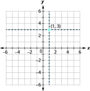
Notice that the vertical line through [latex]x=1[/latex] and the horizontal line through [latex]y=3[/latex] are not part of the graph. We just used them to help us locate the point [latex](1,3)[/latex].
When one of the coordinate is zero, the point lies on one of the axes. In the figure below, the point [latex](0,4)[/latex] is on the y-axis and the point [latex](-2,0)[/latex] is on the x-axis.
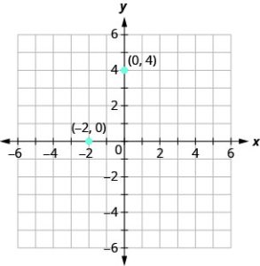
Points on the Axes
Points with a y-coordinate equal to 0 are on the x-axis, and have coordinates [latex](a,0)[/latex].
Points with an x-coordinate equal to 0 are on the y-axis, and have coordinates [latex](0,b)[/latex].
Example 1
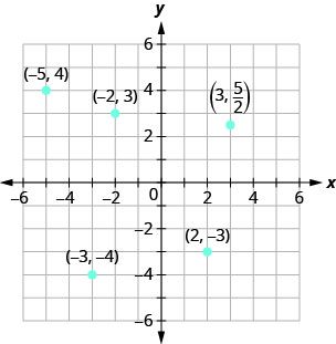
Plot each point in the rectangular coordinate system and identify the quadrant in which the point is located.
(a) [latex](-5,4)[/latex]
The first number of the coordinate pair is the x-coordinate, and the second number is the y-coordinate. To plot each point, sketch a vertical line through the x-coordinate and a horizontal line through the y-coordinate. Their intersection is the point.
Since [latex]x=-5[/latex], the point is to the left of the y-axis. Also, since [latex]y=4[/latex], the point is above the x-axis. The point [latex](-5,4)[/latex] is in Quadrant II.
The graph that shows the plotted point is at the bottom of this example.
(b) [latex](-3,-4)[/latex]
Since [latex]x=-3[/latex] the point is to the left of the y-axis. Also, since [latex]y=-4[/latex] the point is below the x-axis. The point [latex](-3,-4)[/latex] is in Quadrant III.
The graph that shows the plotted point is at the bottom of this example.
(c) [latex](2,-3)[/latex]
Since [latex]x=2[/latex] the point is to the right of the y-axis. Since [latex]y=-3[/latex] the point is below the x-axis. The point [latex](2,-3)[/latex] is in Quadrant IV.
The graph that shows the plotted point is at the bottom of this example.
(d) [latex](-2, 3)[/latex]
Since [latex]x=-2[/latex] the point is to the left of the y-axis. Since [latex]y=3[/latex] the point is above the x-axis. The point [latex](-2, 3)[/latex] is in Quadrant II.
The graph that shows the plotted point is at the bottom of this example.
(e) [latex](3,\frac{5}{2})[/latex]
Since [latex]x=3[/latex] the point is to the right of the y-axis. Since [latex]y=\frac{5}{2}[/latex] the point is above the x-axis. (It may be helpful to write [latex]\frac{5}{2}[/latex] as a mixed number or decimal.) The point [latex](3,\frac{5}{2})[/latex] is in Quadrant I.
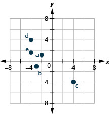
Exercise 1
Plot each point in a rectangular coordinate system and identify the quadrant in which the point is located:
a) [latex](-2,1)[/latex]
b) [latex](-3,-1)[/latex]
c) [latex](4,-4)[/latex]
d) [latex](-4,4)[/latex]
e) [latex](-4,\frac{3}{2})[/latex]
Solution
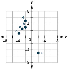
Plot each point in a rectangular coordinate system and identify the quadrant in which the point is located:
a) [latex](-4,1)[/latex]
b) [latex](-2,3)[/latex]
c) [latex](2,-5)[/latex]
d) [latex](-2,5)[/latex]
e) [latex](-3,\frac{5}{2})[/latex]
Solution
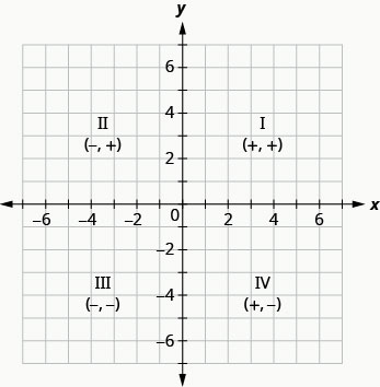
The signs of the x-coordinate and y-coordinate affect the location of the points. You may have noticed some patterns as you graphed the points in the previous example. We can summarize sign patterns of the quadrants in this way:
Quadrants
| Quadrant I | Quadrant II | Quadrant III | Quadrant IV |
| [latex](x,y)[/latex] | [latex](x,y)[/latex] | [latex](x,y)[/latex] | [latex](x,y)[/latex] |
| [latex](+,+)[/latex] | [latex](-,+)[/latex] | [latex](-,-)[/latex] | [latex](+,-)[/latex] |
Up to now, all the equations you have solved were equations with just one variable. In almost every case, when you solved the equation you got exactly one solution. But equations can have more than one variable. Equations with two variables may be of the form [latex]Ax+By=C[/latex]. An equation of this form is called a linear equation in two variables.
Linear Equation
An equation of the form [latex]Ax+By=C[/latex] where A and B are not both zero, is called a linear equation in two variables.
Here is an example of a linear equation in two variables, x and y.
[latex]\begin{eqnarray} Ax+By &=& C\\ x+4y &=& 8\\ A=1, B &=& 4, C=8\\ \end{eqnarray}[/latex]
The equation [latex]y=-3x+5[/latex] is also a linear equation. But it does not appear to be in the form [latex]Ax+By=C[/latex]. We can use the Addition Property of Equality and rewrite it in [latex]Ax+By=C[/latex] form.
[latex]\begin{array}{lrcl} & y & = & -3x+5\\ \text{Add } 3x \text{ to both sides.} & y{+3x} & = & -3x+5{+3x} \\ \text{Simplify.} & y+3x & = & 5\\ \text{Use the Commutative Property to put it in }\\ Ax+By=C \text{ form.} & 3x+y & = & 5\\ \end{array}[/latex]
By rewriting [latex]y=-3x+5[/latex] as [latex]3x+y=5[/latex] we can easily see that it is a linear equation in two variables because it is of the form [latex]Ax+By=C[/latex]. When an equation is in the form [latex]Ax+By=C[/latex] we say it is in standard form of a linear equation.
Standard Form of Linear Equation
A linear equation is in standard form when it is written [latex]Ax+By=C[/latex]
Most people prefer to have A, B, and C be integers and [latex]A\geq0[/latex] when writing a linear equation in standard form, although it is not strictly necessary.
Linear equations have infinitely many solutions. For every number that is substituted for x there is a corresponding y value. This pair of values is a solution to the linear equation and is represented by the ordered pair [latex](x,y)[/latex]. When we substitute these values of x and y into the equation, the result is a true statement, because the value on the left side is equal to the value on the right side.
An ordered pair [latex](x,y)[/latex] is a solution of the linear equation[latex]Ax+By=C[/latex] if the equation is a true statement when the x– and y-values of the ordered pair are substituted into the equation.
Linear equations have infinitely many solutions. We can plot these solutions in the rectangular coordinate system. The points will line up perfectly in a straight line. We connect the points with a straight line to get the graph of the equation. We put arrows on the ends of each side of the line to indicate that the line continues in both directions.
A graph is a visual representation of all the solutions of the equation. It is an example of the saying, “A picture is worth a thousand words.” The line shows you all the solutions to that equation. Every point on the line is a solution of the equation. And, every solution of this equation is on this line. This line is called the graph of the equation. Points not on the line are not solutions!
The graph of a linear equation [latex]Ax+By=C[/latex] is a straight line.
- Every point on the line is a solution of the equation.
- Every solution of this equation is a point on this line.
Example 2
The graph of [latex]y=2x-3[/latex] is shown.
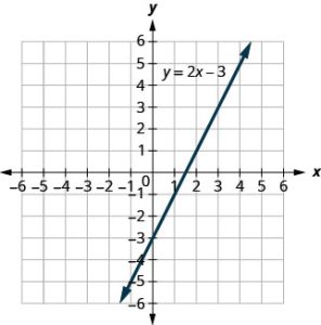
For each ordered pair, decide:
a) Is the ordered pair a solution to the equation?
b) Is the point on the line?
A: [latex](0,-3)[/latex] B: [latex](3,3)[/latex] C: [latex](2,-3)[/latex] D: [latex](-1,-5)[/latex]
Substitute the x– and y-values into the equation to check if the ordered pair is a solution to the equation.
a)
| A: [latex]({0},{-3})[/latex] | B: [latex]({3},{3})[/latex] | C: [latex]({2},{-3})[/latex] | D: [latex]({-1},{-5})[/latex] |
| [latex]\begin{eqnarray} y &=& 2x-3\\ {-3} &\stackrel{?}{=}& 2({0})-3\\ -3 &=& -3\\ \end{eqnarray}[/latex] | [latex]\begin{eqnarray} y &=& 2x-3\\ {3} &\stackrel{?}{=}& 2({3})-3\\ 3 &=& 3\\ \end{eqnarray}[/latex] | [latex]\begin{eqnarray} y &=& 2x-3\\ {-3} &\stackrel{?}{=}& 2({2})-3\\ -3 &\neq& -1\\ \end{eqnarray}[/latex] | [latex]\begin{eqnarray} y &=& 2x-3\\ {-5} &\stackrel{?}{=}& 2({-1})-3\\ -5 &=& -5\\ \end{eqnarray}[/latex] |
| [latex](0,-3)[/latex] is a solution. | [latex](3,3)[/latex] is a solution. | [latex](2,-3)[/latex] is not a solution. | [latex](-1,-5)[/latex] is a solution. |
b) Plot the points [latex](0,-3)[/latex], [latex](3,3)[/latex], [latex](2,-3)[/latex], and [latex](-1,-5)[/latex].
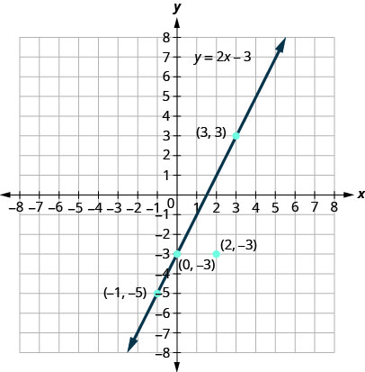
The points [latex](0,-3)[/latex], [latex](3,3)[/latex], and [latex](-1,-5)[/latex] are on the line [latex]y=2x-3[/latex] and the point [latex](2,-3)[/latex] is not on the line.
The points that are solutions to [latex]y=2x-3[/latex] are on the line, but the point that is not a solution is not on the line.
Exercise 2
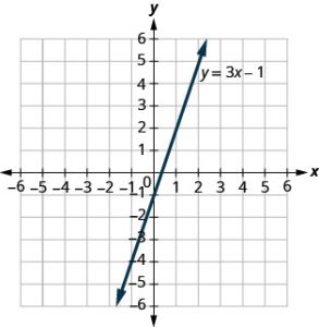
Use graph of [latex]y=3x-1[/latex]. For each ordered pair, decide:
a) Is the ordered pair a solution to the equation?
b) Is the point on the line?
A: [latex](0,-1)[/latex] B: [latex](2,5)[/latex]

Solution
a) yes, yes
b) yes, yes
Use graph of [latex]y=3x-1[/latex]. For each ordered pair, decide:
a) Is the ordered pair a solution to the equation?
b) Is the point on the line?
A: [latex](3,-1)[/latex] B: [latex](-1, -4)[/latex]
Solution
a) no, no
b) yes, yes
Graph a Linear Equation by Plotting Points
There are several methods that can be used to graph a linear equation. The first method we will use is called plotting points, or the Point-Plotting Method. We find three points whose coordinates are solutions to the equation and then plot them in a rectangular coordinate system. By connecting these points in a line, we have the graph of the linear equation.
Example 3
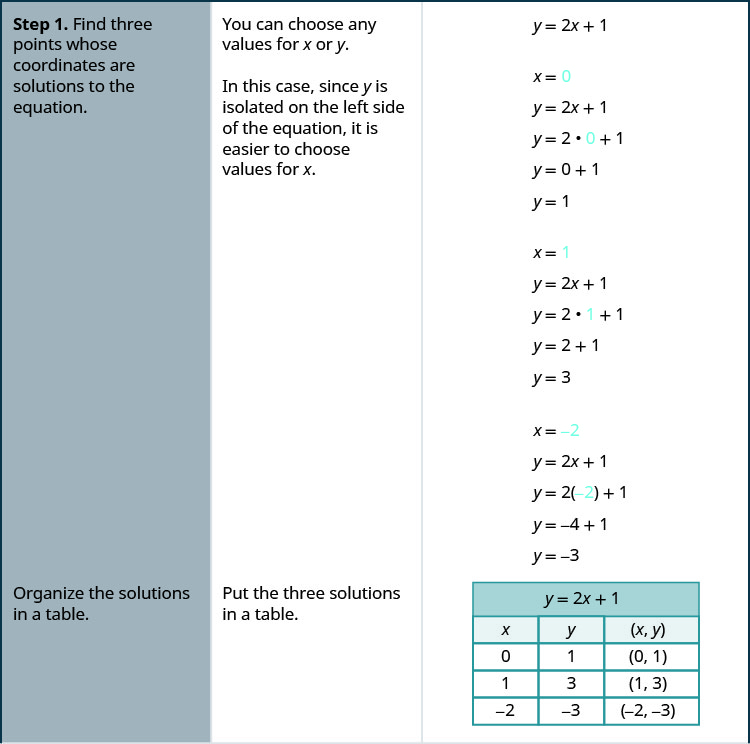
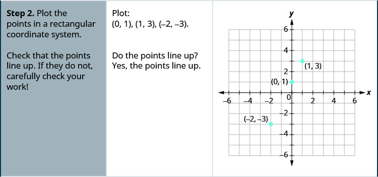
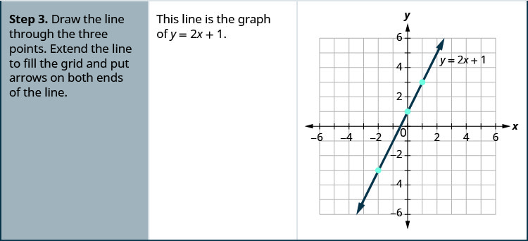
Graph the equation [latex]y=2x+1[/latex] by plotting points.
Exercise 3
Graph the equation by plotting points: [latex]y=2x-3[/latex]. Check your solutions to ensure they are on the line in the graph below.
Solution
Graph the equation by plotting points: [latex]y=-2x+4[/latex]. Check your solutions to ensure they are on the line in the graph below.
Solution
The steps to take when graphing a linear equation by plotting points are summarized here.
- Find three points whose coordinates are solutions to the equation. Organize them in a table.
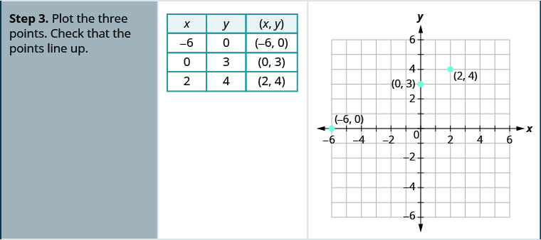
- Plot the points in a rectangular coordinate system. Check that the points line up. If they do not, carefully check your work.
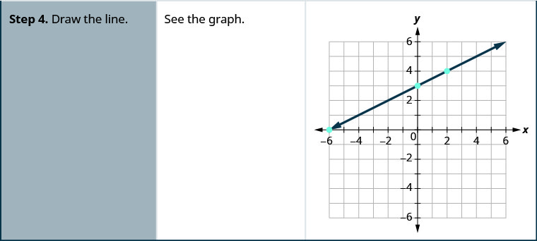
- Draw the line through the three points. Extend the line to fill the grid and put arrows on both ends of the line.
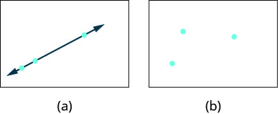
It is true that it only takes two points to determine a line, but it is a good habit to use three points. If you only plot two points and one of them is incorrect, you can still draw a line but it will not represent the solutions to the equation. It will be the wrong line.
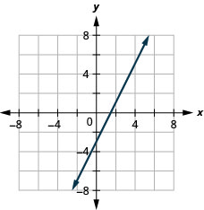
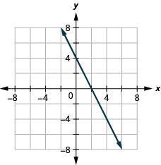
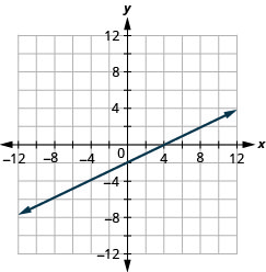
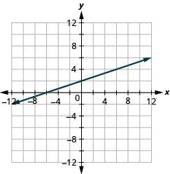
If you use three points, and one is incorrect, the points will not line up. This tells you something is wrong and you need to check your work. Look at the difference between these illustrations.
When an equation includes a fraction as the coefficient of x, we can still substitute any numbers for x. The arithmetic is easier if we make “good” choices for the values of x. Zero is a good choice for the value of x, and multiples of the denominator are good choices, because they will eliminate the fraction. This will avoid fractional answers, which are hard to graph precisely.
Example 4
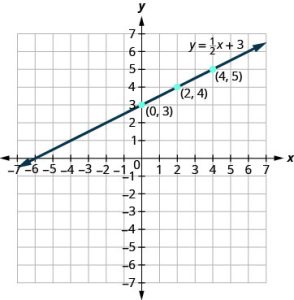
Graph the equation: [latex]y=\frac{1}{2}x+3[/latex].
Find three points that are solutions to the equation. Since this equation has the fraction [latex]\frac{1}{2}[/latex] as a coefficient of x, we will choose values of x carefully. We will use zero as one choice and multiples of 2 for the other choices. Why are multiples of two a good choice for values of x? By choosing multiples of 2 the multiplication by [latex]\frac{1}{2}[/latex] simplifies to a whole number.
| [latex]\begin{eqnarray} x &=& 0\\ y &=& \frac{1}{2}x+3\\ y &=& \frac{1}{2}({0})+3\\ y &=& 0+3\\ y &=& 3\\ \end{eqnarray}[/latex] | [latex]\begin{eqnarray} x &=& 2\\ y &=& \frac{1}{2}x+3\\ y &=& \frac{1}{2}({2})+3\\ y &=& 1+3\\ y &=& 4\\ \end{eqnarray}[/latex] | [latex]\begin{eqnarray} x &=& 4\\ y &=& \frac{1}{2}x+3\\ y &=& \frac{1}{2}({4})+3\\ y &=& 2+3\\ y &=& 5\\ \end{eqnarray}[/latex] |
The points are shown in the figure below.
| [latex]y=\frac{1}{2}x+3[/latex] | ||
| [latex]x[/latex] | [latex]y[/latex] | [latex](x,y)[/latex] |
| [latex]0[/latex] | [latex]3[/latex] | [latex](0,3)[/latex] |
| [latex]2[/latex] | [latex]4[/latex] | [latex](2,4)[/latex] |
| [latex]4[/latex] | [latex]5[/latex] | [latex](4,5)[/latex] |
Plot the points, check that they line up, and draw the line.
Exercise 4
Graph the equation: [latex]y=\frac{1}{3}x-1[/latex].
Solution
Graph the equation: [latex]y=\frac{1}{4}x+2[/latex].
Solution
Graph Vertical and Horizontal Lines
Some linear equations have only one variable. They may have just x and no y, or just y without an x. This changes how we make a table of values to get the points to plot.
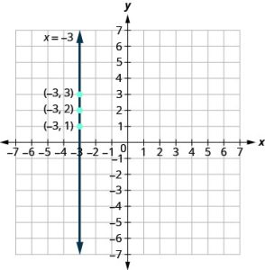
Let’s consider the equation [latex]x=-3[/latex] This equation has only one variable, x. The equation says that x is always equal to[latex]-3[/latex] so its value does not depend on y. Regardless of the value of y, the value of x is always [latex]-3[/latex].
To make a table of values, write [latex]-3[/latex] in for all the x-values, then choose any values for y. We will use 1, 2, and 3 for the y-coordinates.
| [latex]x=-3[/latex] | ||
| [latex]x[/latex] | [latex]y[/latex] | [latex](x,y)[/latex] |
| [latex]-3[/latex] | [latex]1[/latex] | [latex](-3,1)[/latex] |
| [latex]-3[/latex] | [latex]2[/latex] | [latex](-3,2)[/latex] |
| [latex]-3[/latex] | [latex]3[/latex] | [latex](-3,3)[/latex] |
Plot the points from the table and connect them with a straight line. Notice that we have graphed a vertical line passing through the x-axis at [latex]-3[/latex].
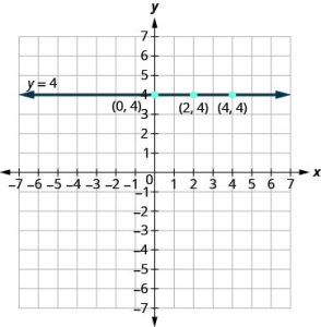
What if the equation has y, but no x? Let’s graph the equation [latex]y=4[/latex] This time the y-value is a constant, so in this equation, y does not depend on x. Fill in 4 for all the y-values in the table, then choose any values for x. We will use 0, 2, and 4 for the x-coordinates.
| [latex]y=4[/latex] | ||
| [latex]x[/latex] | [latex]y[/latex] | [latex](x,y)[/latex] |
| [latex]0[/latex] | [latex]4[/latex] | [latex](0,4)[/latex] |
| [latex]2[/latex] | [latex]4[/latex] | [latex](2,4)[/latex] |
| [latex]4[/latex] | [latex]4[/latex] | [latex](4,4)[/latex] |
In this figure, we have graphed a horizontal line passing through the y-axis at 4.
Vertical and Horizontal Lines
A vertical line is the graph of an equation of the form [latex]x=a[/latex].
 The line passes through the x-axis at [latex](a,0)[/latex].
A horizontal line is the graph of an equation of the form [latex]y=b[/latex].
The line passes through the y-axis at [latex](0,b)[/latex].
Example 5
Graph the following lines.
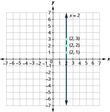
a) [latex]x=2[/latex]
The equation has only one variable, x, and x is always equal to 2. We create a table where x is always 2 and then put in any values for y. The graph is a vertical line passing through the x-axis at 2.
| [latex]x=2[/latex] | ||
| x | y | [latex](x,y)[/latex] |
| 2 | 1 | [latex](2,1)[/latex] |
| 2 | 2 | [latex](2,2)[/latex] |
| 2 | 3 | [latex](2,3)[/latex] |
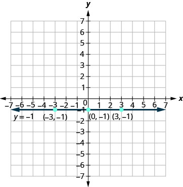
b) [latex]y=-1[/latex]
Similarly, the equation [latex]y=-1[/latex] has only one variable, y. The value of y is constant. All the ordered pairs in the next table have the same y-coordinate. The graph is a horizontal line passing through the y-axis at [latex]-1[/latex].
| [latex]y=-1[/latex] | ||
| x | y | [latex](x,y)[/latex] |
| [latex]0[/latex] | [latex]-1[/latex] | [latex](0,-1)[/latex] |
| [latex]3[/latex] | [latex]-1[/latex] | [latex](3,-1)[/latex] |
| [latex]-3[/latex] | [latex]-1[/latex] | [latex](-3,-1)[/latex] |
Exercise 5
Graph the equations:
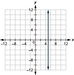
a) [latex]x=5[/latex]
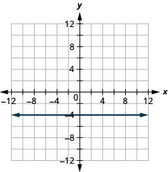
b) [latex]y=-4[/latex]
Solution
a)
b)
Graph the equations:
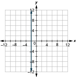
a) [latex]x=-2[/latex]
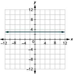
b) [latex]y=3[/latex]
Solution
a)
b)
What is the difference between the equations [latex]y=4x[/latex] and [latex]y=4[/latex]?
The equation [latex]y=4x[/latex] has both x and y. The value of y depends on the value of x, so the y -coordinate changes according to the value of x. The equation [latex]y=4[/latex] has only one variable. The value of y is constant, it does not depend on the value of x, so the y-coordinate is always 4.
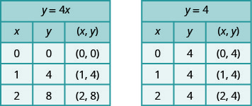
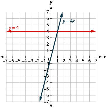
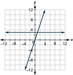
Notice, in the graph, the equation [latex]y=4x[/latex] gives a slanted line, while [latex]y=4[/latex] gives a horizontal line.
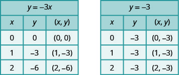
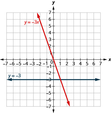
Example 6
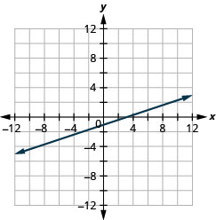
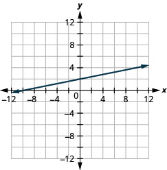
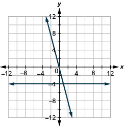
Graph [latex]y=-3x[/latex] and [latex]y=-3[/latex] in the same rectangular coordinate system.
We notice that the first equation has the variable x, while the second does not. We make a table of points for each equation and then graph the lines. The two graphs are shown.
Exercise 6
Graph the equations in the same rectangular coordinate system: [latex]y=-4x[/latex] and [latex]y=-4[/latex].
Solution
Graph the equations in the same rectangular coordinate system: [latex]y=3[/latex] and [latex]y=3x[/latex]
Solution
Find x– and y-intercepts
Every linear equation can be represented by a unique line that shows all the solutions of the equation. We have seen that when graphing a line by plotting points, you can use any three solutions to graph. This means that two people graphing the line might use different sets of three points.
At first glance, their two lines might not appear to be the same, since they would have different points labeled. But if all the work was done correctly, the lines should be exactly the same. One way to recognize that they are indeed the same line is to look at where the line crosses the x-axis and the y-axis. These points are called the intercepts of a line.
The points where a line crosses the x-axis and the y-axis are called the intercepts of the line.
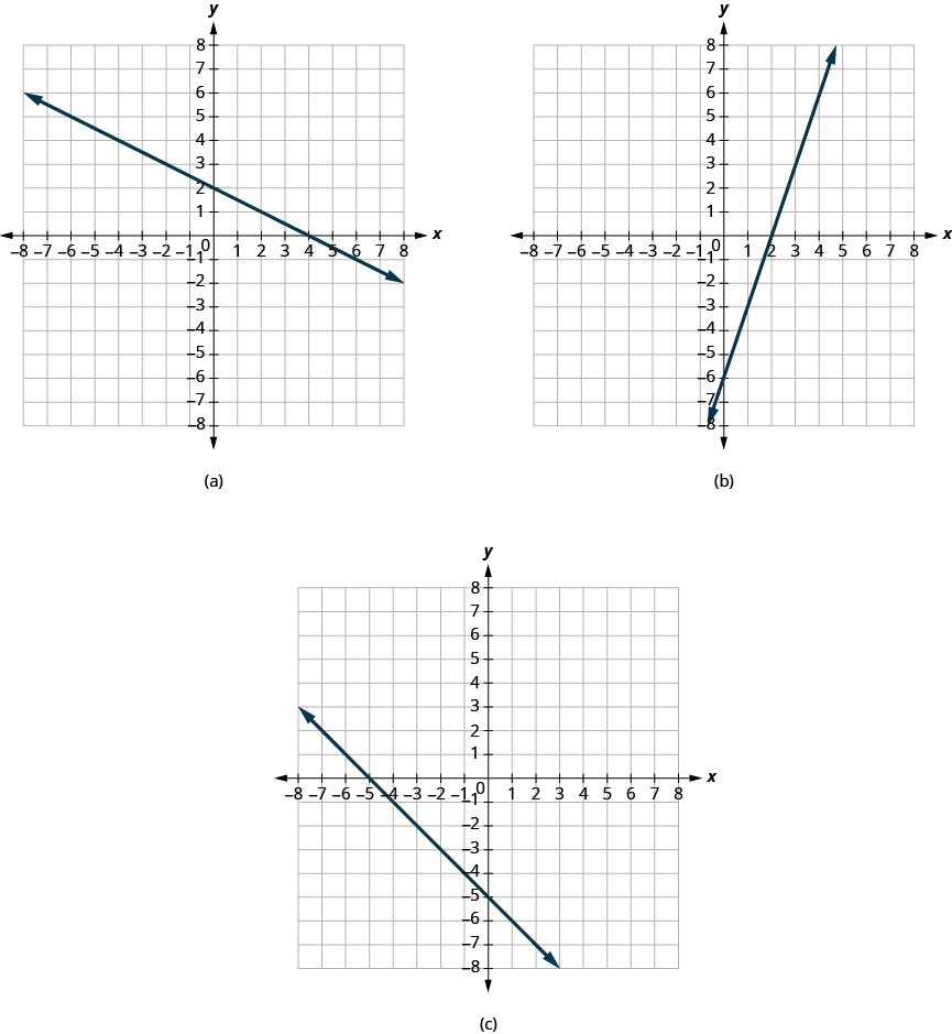
Let’s look at the graphs of the lines.
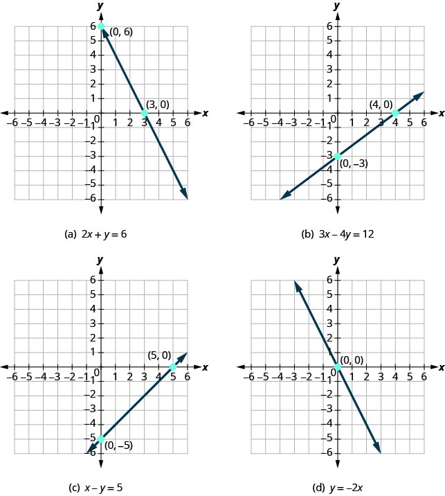
Let’s look at the points where these lines cross the x-axis, and the y-axis.
| Figure | Line crosses x-axis at this point | Line crosses y-axis at this point |
| a | [latex](3,0)[/latex] | [latex](0,6)[/latex] |
| b | [latex](4,0)[/latex] | [latex](0,-3)[/latex] |
| c | [latex](5,0)[/latex] | [latex](0,-5)[/latex] |
| d | [latex](0,0)[/latex] | [latex](0,0)[/latex] |
Do you see a pattern? See the figure below.
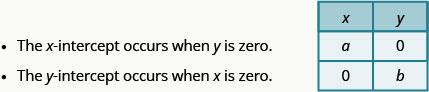
For each line, the y-coordinate of the point where the line crosses the x-axis is zero. The point where the line crosses the x-axis has the form [latex](a,0)[/latex] and is called the x-intercept of the line. The x-intercept occurs when y is zero.
In each line, the x–coordinate of the point where the line crosses the y-axis is zero. The point where the line crosses the y-axis has the form [latex](0,b)[/latex] and is called the y-intercept of the line. The y-intercept occurs when x is zero.
The x-intercept is the point [latex](a,0)[/latex] where the line crosses the x-axis.
The y-intercept is the point [latex](0,b)[/latex] where the line crosses the y-axis.
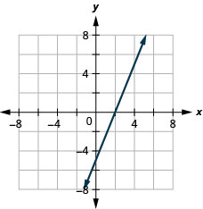
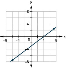
Example 7
Find the x– and y-intercepts on each graph shown.
(a) The graph crosses the x-axis at the point [latex](4,0)[/latex]. The x-intercept is [latex](4,0)[/latex].
The graph crosses the y-axis at the point [latex](0,2)[/latex]. The y-intercept is [latex](0,2)[/latex].
(b) The graph crosses the x-axis at the point [latex](2,0)[/latex]. The x-intercept is [latex](2,0)[/latex].
The graph crosses the y-axis at the point [latex](0,-6)[/latex]. The y-intercept is [latex](0,-6)[/latex].
(c) The graph crosses the x-axis at the point [latex](-5,0)[/latex]. The x-intercept is [latex](-5,0)[/latex].
The graph crosses the y-axis at the point [latex](0,-5)[/latex]. The y-intercept is [latex](0,-5)[/latex].
Exercise 7
Recognizing that the x-intercept occurs when y is zero and that the y-intercept occurs when x is zero, gives us a method to find the intercepts of a line from its equation. To find the x-intercept, let [latex]y=0[/latex] and solve for x. To find the y-intercept, let [latex]x=0[/latex] and solve for y.
Find the x– and y-intercepts from the Equation of a Line
Use the equation of the line to find:
- the x-intercept of the line, let [latex]y=0[/latex] and solve for x.
- the y-intercept of the line, let [latex]x=0[/latex] and solve for y.
Example 8
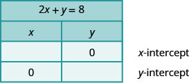
Find the intercepts of [latex]2x+y=8[/latex].
We will let [latex]y=0[/latex] to find the x-intercept, and let [latex]x=0[/latex] to find the y-intercept. Complete the table below.
| [latex]\begin{array}{lrcl} \text{To find the x-intercept, let } y=0.\\ \text {Let } y=0. & 2x+0 & = & 8\\ \text{Simplify.} & 2x & = & 8\\ & x & = & 4\\ \text{The x-intercept is } (4,0). \end{array}[/latex] |
| [latex]\begin{array}{lrcl} \text{To find the y-intercept, let } x=0.\\ \text {Let } x=0. & 2(0)+y & = & 8\\ \text{Simplify.} & 0+y & = & 8\\ & y & = & 8\\ \text{The y-intercept is } (0,8). \end{array}[/latex] |
The intercepts are the points [latex](4,0)[/latex] and [latex](0,8)[/latex] as shown in the table.
| [latex]2x+y=8[/latex] | |
| [latex]x[/latex] | [latex]y[/latex] |
| [latex]4[/latex] | [latex]0[/latex] |
| [latex]0[/latex] | [latex]8[/latex] |
Exercise 8
Graph a Line Using the Intercepts
To graph a linear equation by plotting points, you need to find three points whose coordinates are solutions to the equation. You can use the x- and y- intercepts as two of your three points. Find the intercepts, and then find a third point to ensure accuracy. Make sure the points line up—then draw the line. This method is often the quickest way to graph a line.
Example 9
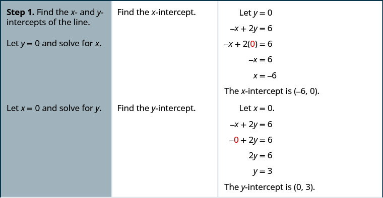
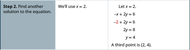
Graph [latex]-x+2y=6[/latex] using the intercepts.
Exercise 9
Graph using the intercepts: [latex]x-2y=4[/latex].
Solution
Graph using the intercepts: [latex]-x+3y=6[/latex].
Solution
The steps to graph a linear equation using the intercepts are summarized here:
- Find the x– and y-intercepts of the line.
- Let [latex]y=0[/latex] and solve for x.
- Let [latex]x=0[/latex] and solve for y.
- Find a third solution to the equation.
- Plot the three points and check that they line up.
- Draw the line.
Example 10
Graph [latex]4x-3y=12[/latex] using the intercepts.
Find the intercepts and a third point.
| x-intercept, let y=0 | y-intercept, let x=0 | third point, let y=4 |
| [latex]\begin{eqnarray} 4x-3y &=& 12\\ 4x-3({0}) &=& 12\\ 4x &=& 12\\ x &=& 3\\ \end{eqnarray}[/latex] | [latex]\begin{eqnarray} 4x-3y &=& 12\\ 4({0})-3y &=& 12\\ -3y &=& 12\\ y &=& -4\\ \end{eqnarray}[/latex] | [latex]\begin{eqnarray} 4x-3y &=& 12\\ 4x-3({4}) &=& 12\\ 4x-12 &=& 12\\ 4x &=& 24\\ x &=& 6\\ \end{eqnarray}[/latex] |
We list the points in the table and show the graph.
| [latex]4x-3y=12[/latex] | ||
| [latex]x[/latex] | [latex]y[/latex] | [latex](x,y)[/latex] |
| [latex]3[/latex] | [latex]0[/latex] | [latex](3,0)[/latex] |
| [latex]0[/latex] | [latex]-4[/latex] | [latex](0,-4)[/latex] |
| [latex]6[/latex] | [latex]4[/latex] | [latex](6,4)[/latex] |
Exercise 10
Graph using the intercepts: [latex]5x-2y=10[/latex].
Solution
Graph using the intercepts: [latex]3x-4y=12[/latex].
Solution
When the line passes through the origin, the x-intercept and the y-intercept are the same point.
Example 11
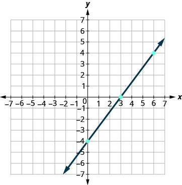
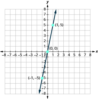
Graph [latex]y=5x[/latex] using the intercepts.
|
x-intercept, let [latex]y=0[/latex]. |
y-intercept, let [latex]x=0[/latex]. |
| [latex]\begin{eqnarray} y &=& 5x\\ {0} &=& 5x\\ 0 &=& x\\ \end{eqnarray}[/latex] | [latex]\begin{eqnarray} y &=& 5x\\ y &=& 5\cdot{0}\\ y &=& 0\\ \end{eqnarray}[/latex] |
|
[latex](0,0)[/latex] |
[latex](0,0)[/latex] |
This line has only one intercept. It is the point [latex](0,0)[/latex].
To ensure accuracy, we need to plot three points. Since the x– and y-intercepts are the same point, we need two more points to graph the line.
|
Let [latex]x=1[/latex]. |
Let [latex]x=-1[/latex]. |
| [latex]\begin{eqnarray} y &=& 5x\\ y &=& 5\cdot{1}\\ y &=& 5\\ \end{eqnarray}[/latex] | [latex]\begin{eqnarray} y &=& 5x\\ y &=& 5{-1}\\ y &=& -5\\ \end{eqnarray}[/latex] |
The resulting three points are summarized in the table.
| [latex]y=5x[/latex] | ||
| [latex]x[/latex] | [latex]y[/latex] | [latex](x,y)[/latex] |
| [latex]0[/latex] | [latex]0[/latex] | [latex](0,0)[/latex] |
| [latex]1[/latex] | [latex]5[/latex] | [latex](1,5)[/latex] |
| [latex]-1[/latex] | [latex]-5[/latex] | [latex](-1,-5)[/latex] |
Plot the three points, check that they line up, and draw the line.
Exercise 11
Graph using the intercepts: [latex]y=4x[/latex].
Solution

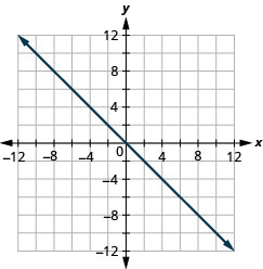
Graph the intercepts: [latex]y=-x[/latex].
Solution
Media Attributions
- 1.3.1 © OpenStax Intermediate Algebra 2e is licensed under a CC BY (Attribution) license
- 1.3.2 © OpenStax Intermediate Algebra 2e is licensed under a CC BY (Attribution) license
- 1.3.3 © OpenStax Intermediate Algebra 2e is licensed under a CC BY (Attribution) license
- 1.3.4 © OpenStax Intermediate Algebra 2e is licensed under a CC BY (Attribution) license
- 1.3.5 © OpenStax Intermediate Algebra 2e is licensed under a CC BY (Attribution) license
- 1.3.6 © OpenStax Intermediate Algebra 2e is licensed under a CC BY (Attribution) license
- 1.3.7 © OpenStax Intermediate Algebra 2e is licensed under a CC BY (Attribution) license
- 1.3.8 © OpenStax Intermediate Algebra 2e is licensed under a CC BY (Attribution) license
- 1.3.9 © OpenStax Intermediate Algebra 2e is licensed under a CC BY (Attribution) license
- 1.3.10 © OpenStax Intermediate Algebra 2e is licensed under a CC BY (Attribution) license
- 1.3.11 © OpenStax Intermediate Algebra 2e is licensed under a CC BY (Attribution) license
- 1.3.12 © OpenStax Intermediate Algebra 2e is licensed under a CC BY (Attribution) license
- 1.3.13 © OpenStax Intermediate Algebra 2e is licensed under a CC BY (Attribution) license
- 1.3.14 © OpenStax Intermediate Algebra 2e is licensed under a CC BY (Attribution) license
- 1.3.15 © OpenStax Intermediate Algebra 2e is licensed under a CC BY (Attribution) license
- 1.3.16 © OpenStax Intermediate Algebra 2e is licensed under a CC BY (Attribution) license
- 1.3.17 © OpenStax Intermediate Algebra 2e is licensed under a CC BY (Attribution) license
- 1.3.18 © OpenStax Intermediate Algebra 2e is licensed under a CC BY (Attribution) license
- 1.3 19 © OpenStax Intermediate Algebra 2e is licensed under a CC BY (Attribution) license
- 1.3.20 © OpenStax Intermediate Algebra 2e is licensed under a CC BY (Attribution) license
- 1.3.21 © OpenStax Intermediate Algebra 2e is licensed under a CC BY (Attribution) license
- 1.3.22 © OpenStax Intermediate Algebra 2e is licensed under a CC BY (Attribution) license
- 1.3.23 © OpenStax Intermediate Algebra 2e is licensed under a CC BY (Attribution) license
- 1.3.24 © OpenStax Intermediate Algebra 2e is licensed under a CC BY (Attribution) license
- 1.3.25 © OpenStax Intermediate Algebra 2e is licensed under a CC BY (Attribution) license
- 1.3.26 © OpenStax Intermediate Algebra 2e is licensed under a CC BY (Attribution) license
- 1.3.27 © OpenStax Intermediate Algebra 2e is licensed under a CC BY (Attribution) license
- 1.3.28 © OpenStax Intermediate Algebra 2e is licensed under a CC BY (Attribution) license
- 1.3.29 © OpenStax Intermediate Algebra 2e is licensed under a CC BY (Attribution) license
- 1.3.30 © OpenStax Intermediate Algebra 2e is licensed under a CC BY (Attribution) license
- 1.3.31 © OpenStax Intermediate Algebra 2e is licensed under a CC BY (Attribution) license
- 1.3.32 © OpenStax Intermediate Algebra 2e is licensed under a CC BY (Attribution) license
- 1.3.33 © OpenStax Intermediate Algebra 2e is licensed under a CC BY (Attribution) license
- 1.3.34 © OpenStax Intermediate Algebra 2e is licensed under a CC BY (Attribution) license
- 1.3.35 © OpenStax Intermediate Algebra 2e is licensed under a CC BY (Attribution) license
- 1.3.36 © OpenStax Intermediate Algebra 2e is licensed under a CC BY (Attribution) license
- 1.3.37 © OpenStax Intermediate Algebra 2e is licensed under a CC BY (Attribution) license
- 1.3.38 © OpenStax Intermediate Algebra 2e is licensed under a CC BY (Attribution) license
- 1.3.41 © OpenStax Intermediate Algebra 2e is licensed under a CC BY (Attribution) license
- 1.3.42 © OpenStax Intermediate Algebra 2e is licensed under a CC BY (Attribution) license
- 1.3.43 © OpenStax Intermediate Algebra 2e is licensed under a CC BY (Attribution) license
- 1.3.44 © OpenStax Intermediate Algebra 2e is licensed under a CC BY (Attribution) license
- 1.3.45 © OpenStax Intermediate Algebra 2e is licensed under a CC BY (Attribution) license
- 1.3.46 © OpenStax Intermediate Algebra 2e is licensed under a CC BY (Attribution) license
- 1.3.47 © OpenStax Intermediate Algebra 2e is licensed under a CC BY (Attribution) license
- 1.3.48 © OpenStax Intermediate Algebra 2e is licensed under a CC BY (Attribution) license
- 1.3.49 © OpenStax Intermediate Algebra 2e is licensed under a CC BY (Attribution) license
- 1.3.50 © OpenStax Intermediate Algebra 2e is licensed under a CC BY (Attribution) license
- 1.3.51 © OpenStax Intermediate Algebra 2e is licensed under a CC BY (Attribution) license
- 1.3.52 © OpenStax Intermediate Algebra 2e is licensed under a CC BY (Attribution) license
- 1.3.53 © OpenStax Intermediate Algebra 2e is licensed under a CC BY (Attribution) license
A grid system used in algebra to show a relationship between two variables and formed by intersecting one horizontal line, called the x-axis, with a vertical line, called the y-axis.
The horizonal number line that intersects with a vertical number line to form the rectangular coordinate system.
The vertical number line that intersects with a horizontal number line to form the rectangular coordinate system.
The four regions formed by the intersecting x- and y-axes,
An ordered pair, [latex](x,y)[/latex] gives the coordinates of a point in a rectangular coordinate system. The first number is the x-coordinate. The second number is the y-coordinate.
The first number in an ordered pair.
The second number in an ordered pair.
The point [latex](0,0)[/latex] is called the origin. It is the point where the x-axis and y-axis intersect.
A vertical line is the graph of an equation of the form [latex]x=a[/latex] The line passes through the x-axis at [latex](a,0)[/latex].
A horizontal line is the graph of an equation of the form [latex]y=b[/latex] The line passes through the y-axis at [latex](0,b)[/latex].
An equation of the form [latex]Ax+By=C[/latex] where A and B are not both zero, is called a linear equation in two variables.
A linear equation is in standard form when it is written [latex]Ax+By=C[/latex].
An ordered pair [latex](x,y)[/latex] is a solution of the linear equation[latex]Ax+By=C[/latex] if the equation is a true statement when the x– and y-values of the ordered pair are substituted into the equation.
A solution is a value of a variable that makes a true statement when substituted into the equation.
a visual representation of all the solutions of the equation
The points where a line crosses the x-axis and the y-axis are called the intercepts of the line.
