Chapter 8 Statistics
8.7 Scatter Plots, Correlation, and Regression Lines
Learning Objectives
By the end of this section, you will be able to:
- Construct a scatter plot for a dataset
- Interpret a scatter plot
- Distinguish among positive, negative, and no correlation
- Compute the correlation coefficient
- Estimate and interpret regression lines
One of the most powerful tools statistics gives us is the ability to explore relationships between two datasets containing quantitative values and then use that relationship to make predictions. For example, a student who wants to know how well they can expect to score on an upcoming final exam may consider reviewing the data on midterm and final exam scores for students who have previously taken the class. It seems reasonable to expect that there is a relationship between those two datasets: If a student did well on the midterm, they were probably more likely to do well on the final than the average student. Similarly, if a student did poorly on the midterm, they probably also did poorly on the final exam.
Of course, that relationship isn’t set in stone; a student’s performance on a midterm exam doesn’t cement their performance on the final! A student might use a poor result on the midterm as motivation to study more for the final. A student with a really good grade on the midterm might be overconfident going into the final and as a result won’t prepare adequately.
The statistical method of regression can find a formula that does the best job of predicting a score on the final exam based on the student’s score on the midterm as well as give a measure of the confidence of that prediction! In this section, we’ll discover how to use regression to make these predictions. First, though, we need to lay some graphical groundwork.
Relationships between Quantitative Datasets
Before we can evaluate a relationship between two datasets, we must first decide if we feel that one might depend on the other. In our exam example, it is appropriate to say that the score on the final depends on the score on the midterm rather than the other way around: if the midterm depended on the final, then we’d need to know the final score first, which doesn’t make sense.
Here’s another example: if we collected data on home purchases in a certain area and noted both the sale price of the house and the annual household income of the purchaser, we might expect a relationship between those two. Which depends on the other? In this case, sale price depends on income: people who have a higher income can afford a more expensive house. If it were the other way around, people could buy a new, more expensive house and then expect a raise! (This is very bad advice.)
It’s worth noting that not every pair of related datasets has clear dependence. For example, consider the percent of a country’s budget devoted to the military and the percent earmarked for public health. These datasets are generally related: as one goes up, the other goes down. However, in this case, there’s not a preferred choice for dependence, as each could be seen as depending on the other. When exploring the relationship between two datasets, if one set seems to depend on the other, we’ll say that dataset contains values of the response variable (or dependent variable). The dataset that the response variable depends on contains values of what we call the explanatory variable (or independent variable). If no dependence relationship can be identified, then we can assign either dataset to either role.
Example 1
For each of the following pairs of related datasets, identify which (if any) should be assigned the role of response variable and which should be assigned to be the explanatory variable.
a) A person’s height and weight
As people get taller, their weight tends to increase. But if a person goes on a diet and loses weight, we don’t expect them to also get shorter. So weight depends on height. That means we’ll say that the response variable is weight and the explanatory variable is height.
b) A professional basketball player’s salary and their average points scored per game (which is a measure of how good they are at basketball)
The more points a basketball player scores, the more money they should make. But if a basketball player gets a raise, we wouldn’t expect them to get better at basketball as a result. So the response is salary and the explanatory is points per game.
c) The length and width of leaves on a tree
The way that the length and width of leaves are connected isn’t clear. It seems reasonable that as the width goes up, so would the length. But the other direction is also plausible: as the length goes up, so does the width. Without a clear dependence relationship, we’re free to declare either to be the response and the other to be the explanatory.
Exercise 1
Given these pairs of datasets, identify which (if either) would be the best choice for the response variable.
a) A person’s age and their annual income
b) A student’s GPA and their score on the ACT
c) A student’s GPA and the number of hours they spend studying per week
Solution
a) Income
b) Either; neither one seems to directly influence the other (they’re both influenced by the student’s academic ability)
c) GPA
Once we’ve assigned roles to our two datasets, we can take the first step in visualizing the relationship between them: creating a scatter plot.
Creating Scatter Plots
A scatter plot is a visualization of the relationship between two quantitative sets of data. The scatter plot is created by turning the datasets into ordered pairs: the first coordinate contains data values from the explanatory dataset, and the second coordinate contains the corresponding data values from the response dataset. These ordered pairs are then plotted in the [latex]xy[/latex]-plane. Let’s return to our exam example to put this into practice.
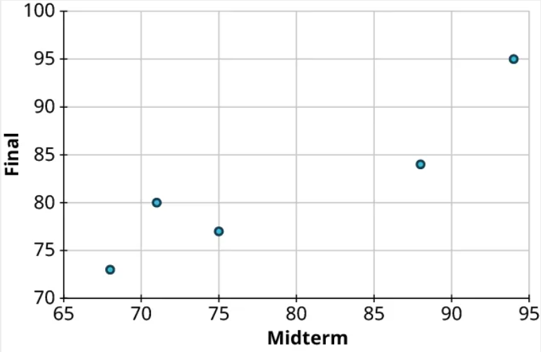
Example 2
Students are exploring the relationship between scores on the midterm exam and final exam in their math course. Here are some of the scores reported by their classmates:
| Name | Midterm grade | Final grade |
| Student 1 | 88 | 84 |
| Student 2 | 71 | 80 |
| Student 3 | 75 | 77 |
| Student 4 | 94 | 95 |
| Student 5 | 68 | 73 |
Create a scatter plot to visualize the data.
Step 1: Since it makes more sense to think of the final exam score as being dependent on the midterm exam score, we’ll let the final grade be the response. So let’s think of these two datasets as a set of ordered pairs, midterm first, final second:
| Name | (Midterm, final) |
|---|---|
| Student 1 | (88, 84) |
| Student 2 | (71, 80) |
| Student 3 | (75, 77) |
| Student 4 | (94, 95) |
| Student 5 | (68, 73) |
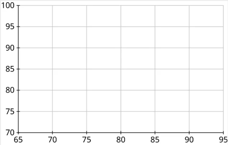
Step 2: Next, let’s make the axes. On the horizontal axis, make sure the range of values is sufficient to cover all of the explanatory data. For our data, that’s 68 to 94. Similarly, the vertical axis should cover all of the response data (73 to 95):
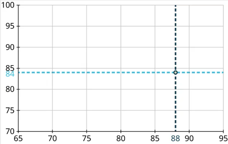
Step 3: Our first point is (88, 84). So we’ll locate 88 on the horizontal axis and 84 on the vertical axis and identify the point that’s directly above the first location and horizontally level with the second:
Step 4: Repeat this process to place the other four points on the graph:
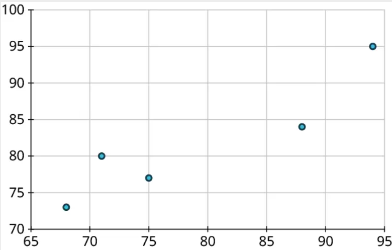
Step 5: Finally, label the axes:
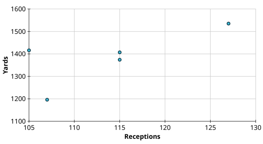
Exercise 2
Create a scatter plot to visualize the following data, showing the top five NFL receivers by number of receptions for the 2019 season. Treat Yards as the response:
| Player | Receptions | Yards |
|---|---|---|
| Stefon Diggs | 127 | 1535 |
| Davante Adams | 115 | 1374 |
| DeAndre Hopkins | 115 | 1407 |
| Darren Waller | 107 | 1196 |
| Travis Kelce | 105 | 1416 |
Solution
Reading and Interpreting Scatter Plots
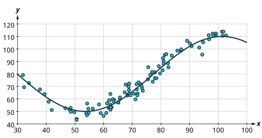
Scatter plots give us information about the existence and strength of a relationship between two datasets. To break that information down, there are a series of questions we might ask to help us. First: Is there a curved pattern in the data? If the answer is “yes,” then we can stop; none of the linear regression techniques from here to the end of this section are appropriate. Figure 7 and Figure 9 show several examples of scatter plots that can help us identify these curved patterns.
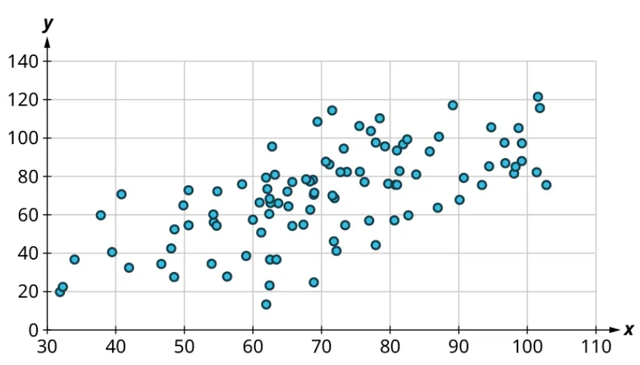
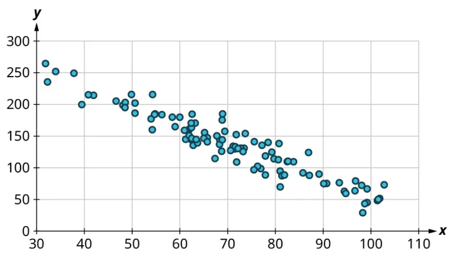
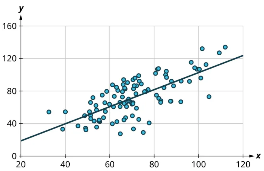
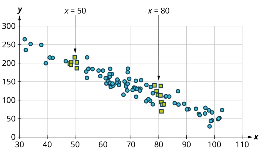
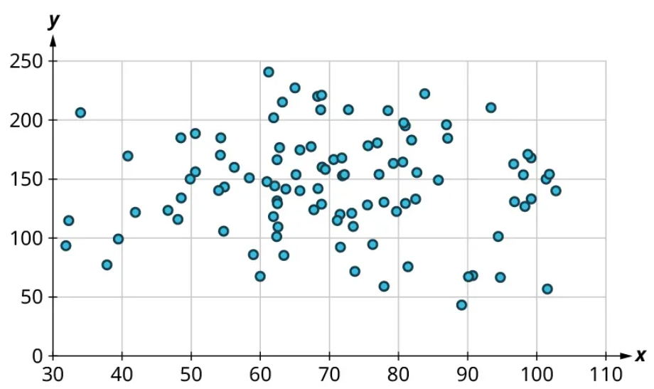
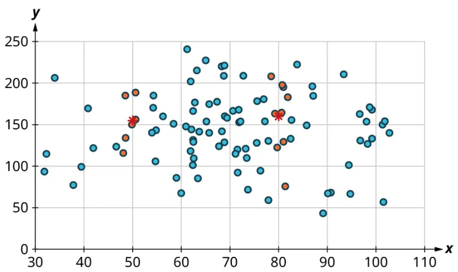
Once we have confirmed that there is no curved pattern in our data, we can move to the next question: Is there a linear relationship? To answer this, we must look at different values of the explanatory variable and determine whether the corresponding response values are different on average. It’s important to look at the values “on average” because, in general, our scatter plots won’t include just one corresponding response point for each value of the explanatory variable (i.e., there may be multiple response values for each explanatory value). So we try to look for the center of those points. Let’s look again at Figure 10 but consider some different values for the explanatory variable. Let’s highlight the points whose [latex]x[/latex]-values are around 50 and those that are around 80:
Now, we can estimate the middle of each group of points. Let’s add our estimated averages to the plot as starred points:
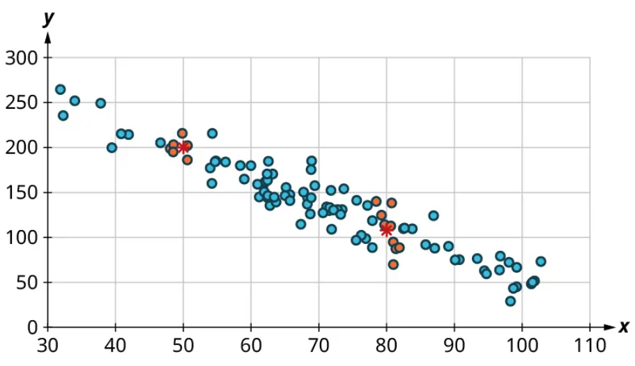
Since those two starred points occur at different heights, we can conclude that there’s likely a relationship worth exploring.
Here’s another example using a different set of data:
Let’s look again at the points near 50 and near 80 and estimate the middles of those clusters:
Notice that there’s not much vertical distance between our two starred points. This tells us that there’s not a strong relationship between these two datasets.
Positive and Negative Linear Relationships
Another way to assess whether there is a relationship between two datasets in a scatter plot is to see if the points seem to be clustered around a line (specifically, a line that’s not horizontal). The stronger the clustering around that line is, the stronger the relationship.
Once we’ve established that there’s a relationship worth exploring, it’s time to start quantifying that relationship. Two datasets have a positive linear relationship if the values of the response tend to increase, on average, as the values of the explanatory variable increase. If the values of the response decrease with increasing values of the explanatory variable, then there is a negative linear relationship between the two datasets. The strength of the relationship is determined by how closely the scatter plot follows a single straight line: the closer the points are to that line, the stronger the relationship. The scatter plots in Figure 15 to Figure 21 depict varying strengths and directions of linear relationships.

The strength and direction (positive or negative) of a linear relationship can also be measured with a statistic called the correlation coefficient (denoted [latex]r[/latex]). Positive values of [latex]r[/latex] indicate a positive relationship, while negative values of [latex]r[/latex] indicate a negative relationship. Values of [latex]r[/latex] close to 0 indicate a weak relationship, while values close to [latex]\pm{1}[/latex] correspond to a very strong relationship. Looking again at Figure 15 to Figure 21, the correlation coefficients for each, in sequential order, are ‒1, ‒0.97, ‒0.55, ‒0.03, 0.61, 0.97, and 1.
There’s no firm rule that establishes a cutoff value of [latex]r[/latex] to divide strong relationships from weak ones, but [latex]\pm{0.7}[/latex] is often given as the dividing line (i.e., if [latex]r > 0.7[/latex] or [latex]r −0.7[/latex], the relationship is strong, and if [latex]−0.7 r 0.7[/latex], the relationship is weak). The formula for computing [latex]r[/latex] is very complicated; it’s almost never done without technology. In this book, we will not compute [latex]r[/latex] but instead will approximate it based on the shape of the scatterplots. In future statistics courses, you may learn how to use technology to compute [latex]r[/latex]. Let’s put all of this together in an example.
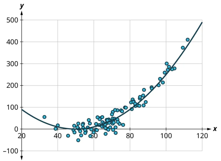
Example 3
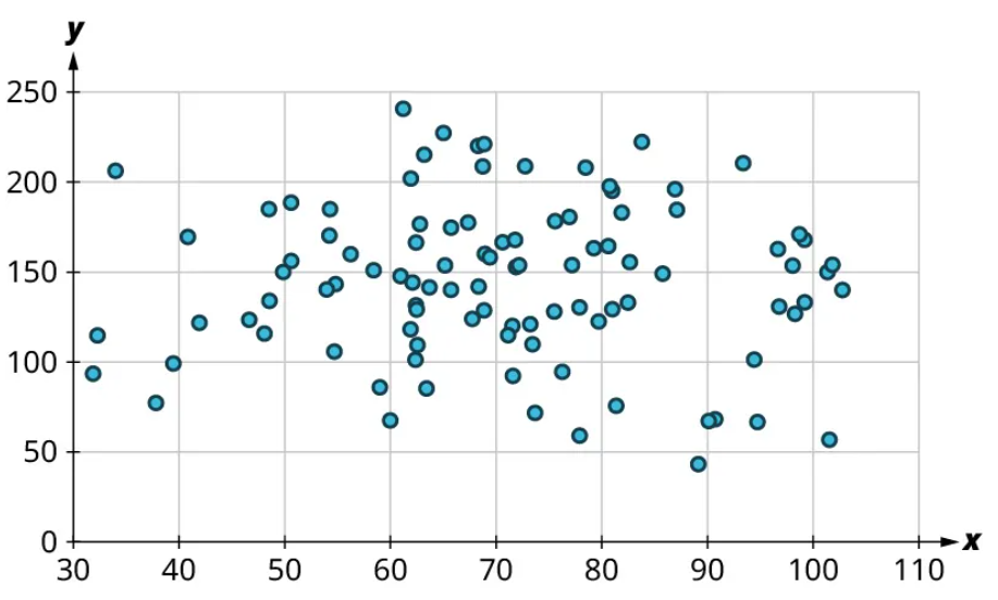
Consider the four scatter plots below. For each of these, answer the following questions:
(1) Is there a curved pattern in the data? If yes, stop here. If no, continue to part b.
(2) Classify the strength and direction of the relationship. Make a guess at the value of [latex]r[/latex].
a)
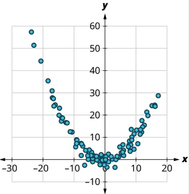
(1) Yes, there is a curved pattern.
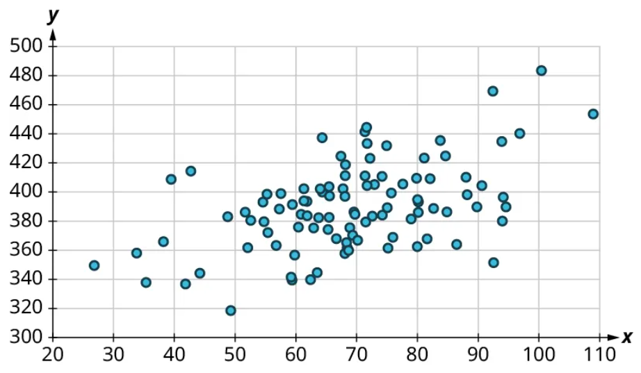
b)
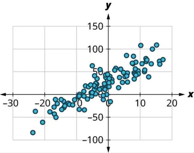
(1) No, there’s no curved pattern.
(2) Since the points trend upward as we move from left to right, this is a positive relationship. The points seem pretty closely grouped around a line, so it’s fairly strong. Comparing this scatter plot to those in Figure 15 to Figure 21, we can see that the relationship is stronger than the one in Figure 19 ([latex]r=0.61[/latex]) but not as strong as the one in Figure 16 ([latex]r=0.97[/latex]). So the value of the correlation coefficient is somewhere between the two. We might guess that [latex]r=0.9[/latex].
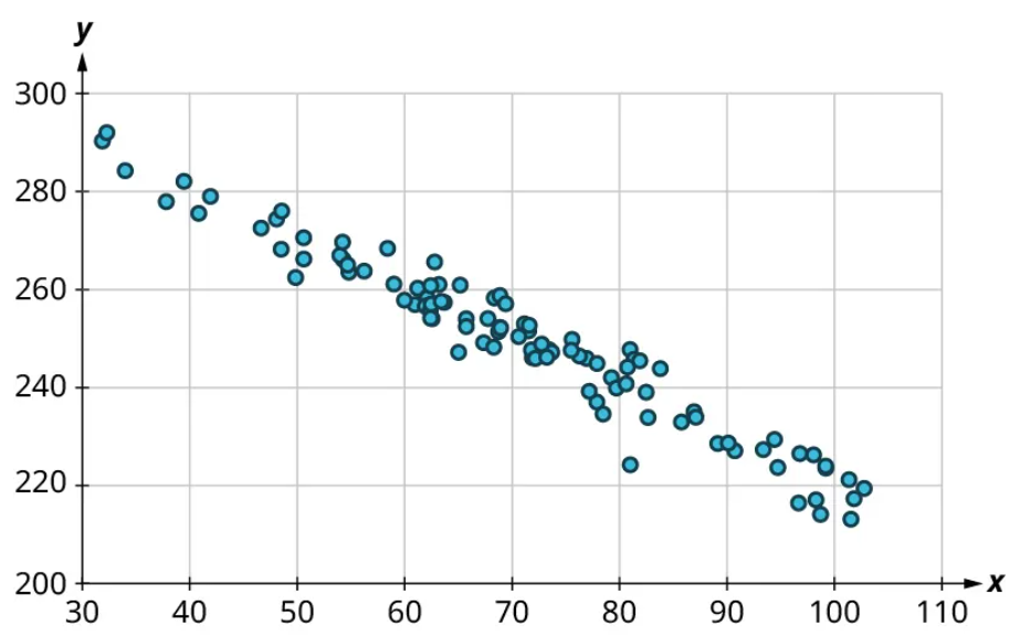
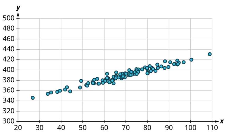
c)
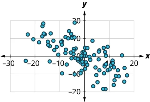
(1) No, there’s no curved pattern.
(2) Since the points tend downward as we move from left to right, this is a negative relationship. The points are not tightly grouped around a line, but the pattern is clear. It looks like it has approximately the same strength as the plot in Figure 19, just with the opposite sign. So we might guess that [latex]r=-0.6[/latex].
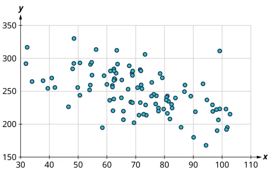
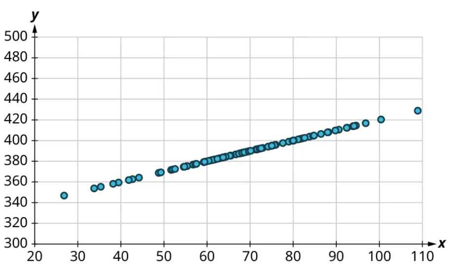
d)
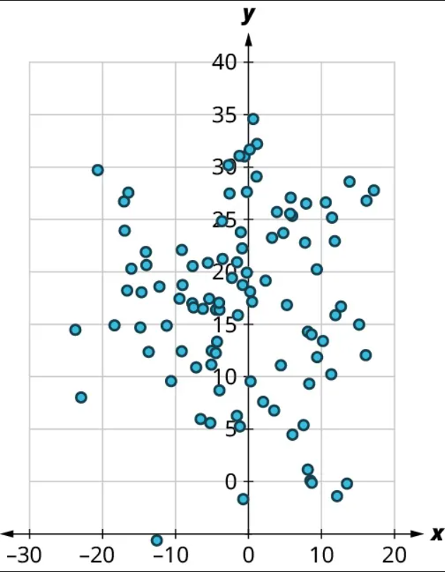
(1) No, there’s no curved pattern.
(2) Since the points don’t really tend upward or downward as we move from left to right, there is no real relationship here. Thus, [latex]r \approx{0}[/latex].
Exercise 3
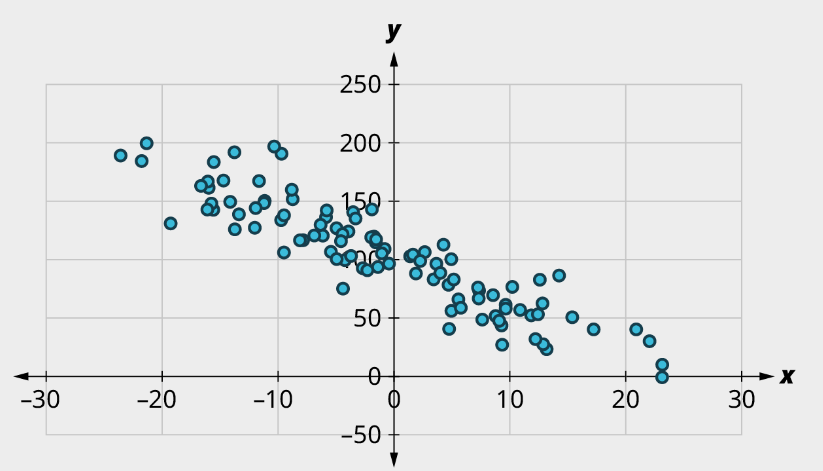
For each of the plots below, answer the following questions:
(1) Is there a curved pattern in the data? If yes, stop here. If no, continue to part b.
(2) Classify the strength and direction of the relationship. Make a guess at the value of r.
a)
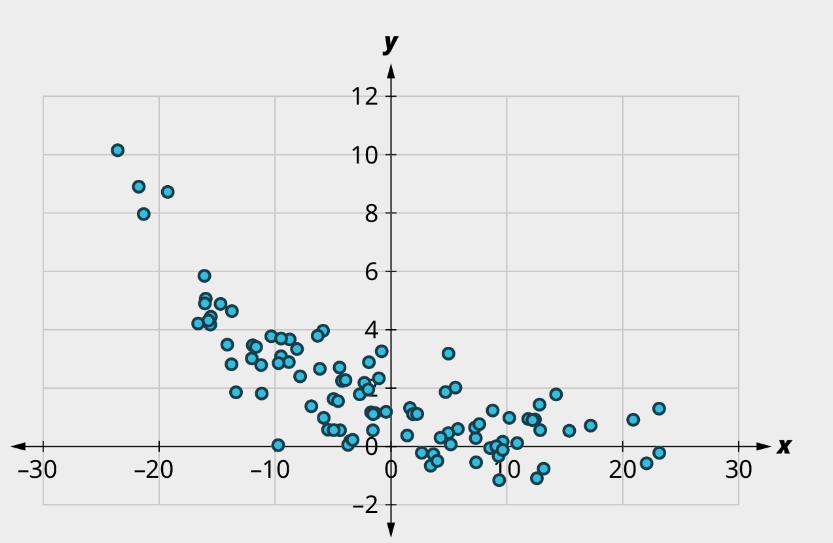
b)
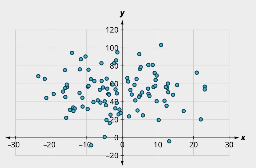
c)
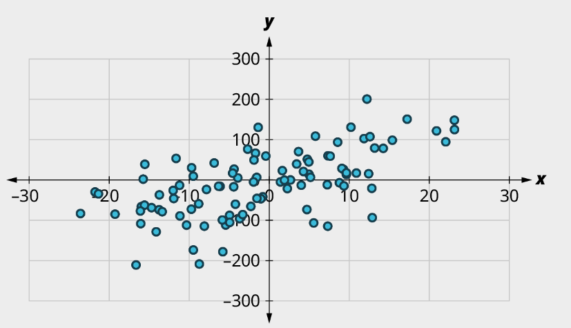
d)
Solution
a) (1) No curved pattern; (2) Strong negative relationship, [latex]r \approx{-0.9}[/latex]
b) (1) Curved pattern
c) (1) No curved pattern; (2) Strong apparent relationship, [latex]r \approx{0}[/latex]
d) (1) No curved pattern; (2) Weak Positive relationship, [latex]r \approx{0.6}[/latex]
Linear Regression
The final step in our analysis of the relationship between two datasets is to find and use the equation of the regression line. For a given set of explanatory and response data, the regression line (also called the least-squares line or line of best fit) is the line that does the best job of approximating the data.
What does it mean to say that a particular line does the “best job” of approximating the data? The way that statisticians characterize this “best line” is rather technical, but we’ll include it for the sake of satisfying your curiosity (and backing up the claim of “best”). Imagine drawing a line that looks like it does a pretty good job of approximating the data. Most of the points in the scatter plot will probably not fall exactly on the line; the distance above or below the line a given point falls on is called that point’s residual. We could compute the residuals for every point in the scatter plot. If you take all those residuals and square them, then add the results together, you get a statistic called the sum of squared errors for the line (the name tells you what it is: “sum” because we’re adding, “squared” because we’re squaring, and “errors” is another word for “residuals”). The line that we choose to be the “best” is the one that has the smallest possible sum of squared errors. The implied minimization (“smallest”) is where the “least” in “least squares” comes from; the “squares” comes from the fact that we’re minimizing the sum of squared errors. This is very similar to the process we outlined in the “game” that we used to introduce the mean. Both the regression line and the mean are designed to minimize a sum of squared errors. Here ends the supertechnical part.
Finding the Equation of the Regression Line
So how do we find the equation of the regression line? Recall the point-slope form of the equation of a line:
FORMULA
If a line has slope [latex]m[/latex] and passes through a point [latex](x_0, y_0)[/latex], then the point-slope form of the equation of the line is
[latex]y=m(x-x_0)+y_0[/latex].
The regression line has two properties that we can use to find its equation. First, it always passes through the point of means. If [latex]\bar{x}[/latex] and [latex]\bar{y}[/latex] are the means of the explanatory and response datasets, respectively, then the point of means is [latex](\bar{x}, \bar{y})[/latex]. We’ll use that as the point in the point-slope form of the equation. Second, if [latex]s_{x}[/latex] and [latex]s_{y}[/latex] are the standard deviations of the explanatory and response datasets, respectively, and if [latex]r[/latex] is the correlation coefficient, then the slope is [latex]m=r \times \frac{s_{y}}{s_{x}}[/latex]. Putting all that together with the point-slope formula gives us this:
FORMULA
Suppose [latex]x[/latex] and [latex]y[/latex] are explanatory and response datasets that have a linear relationship. If their means are [latex]\bar{x}[/latex] and [latex]\bar{y}[/latex] respectively, their standard deviations are [latex]s_{x}[/latex] and [latex]s_{y}[/latex], and their correlation coefficient is [latex]r[/latex], then the equation of the regression line is
[latex]y=r \left( \frac{s_y}{s_x} \right) (x-\bar{x})+ \bar{y}[/latex].
Let’s walk through an example.
Example 4
Suppose you have datasets [latex]x[/latex] and [latex]y[/latex] with the following statistics: [latex]x[/latex] has mean 21 and standard deviation 4, [latex]y[/latex] has mean 8 and standard deviation 2, and their correlation coefficient is −0.4. What’s the equation of the regression line?
Step 1: We’re given [latex]\bar{x}=21[/latex], [latex]s_x =4[/latex], [latex]\bar{y}=8[/latex], [latex]s_y=2[/latex], and [latex]r=-0.4[/latex]. Let’s start with the formula for the equation of the regression line:
[latex]y=r \left( \frac{s_y}{s_x} \right) (x-\bar{x})+ \bar{y}[/latex].
Step 2: Plugging in our values gives us
[latex]y=-0.4 \left( \frac{2}{4} \right) (x-21)+8[/latex].
Step 3: Our final regression line equation is
[latex]y= -0.2x+12.2[/latex].
Exercise 4
Suppose you have datasets x and y with the following statistics: x has mean 100 and standard deviation 5, y has mean 200 and standard deviation 20, and their correlation coefficient is 0.75. What’s the equation of the regression line?
Solution
[latex]y=3x-100[/latex]
Correlation coefficient and linear regression equations can easily be found with a program like Desmos. Here is a video that explains how to use the technology:
Using the Equation of the Regression Line
Once we’ve found the equation of the regression line, what do we do with it? We’ll look at two possible applications: making predictions and interpreting the slope.
We can use the equation of the regression line to predict the response value [latex]y[/latex] for a given explanatory value [latex]x[/latex]. All we have to do is plug that explanatory value into the formula and see what response value results. This is useful in two ways: First, it can be used to make a guess about an unknown data value (like one that hasn’t been observed yet). Second, it can be used to evaluate performance (meaning we can predict an outcome given a particular event). We previously created a scatter plot of final exam scores versus midterm exam scores using these data:
| Name | Midterm grade | Final grade |
| Allison | 88 | 84 |
| Benjamin | 71 | 80 |
| Carly | 75 | 77 |
| Daniel | 94 | 95 |
| Elmo | 68 | 73 |
The equation of the regression line is [latex]y=0.687x+27.4[/latex], where [latex]y[/latex] is the final exam score and [latex]x[/latex] is the midterm exam score. If Frank scored 85 on the midterm, then our prediction for his final exam score is [latex]0.687 \times 85+27.4=85.795[/latex]. To use the regression line to evaluate performance, we use a data value we’ve already observed. For example, Allison scored 88 on the midterm. The regression line predicts that someone who scores an 88 on the midterm will get [latex]0.687 \times 88+27.4=87.856[/latex] on the final. Allison actually scored 84 on the final, meaning she underperformed expectations by almost 4 points [latex](87.856-84)[/latex].
The second application of the equation of the regression line is interpreting the slope of the line to describe the relationship between the explanatory and response datasets. For the exam data in the previous paragraph, the slope of the regression line is 0.687. Recall that the slope of a line can be computed by finding two points on the line and dividing the difference in the [latex]y[/latex]-values of those points by the difference in the [latex]x[/latex]-values. Keeping that in mind, we can interpret our slope as [latex]0.687=\frac{ \text{difference in final scores}}{\text{difference in midterm scores}}[/latex]. Multiplying both sides of that equation by the denominator of the fraction, we get [latex]0.687 \times \text{difference in midterm scores} = \text{difference in final scores}[/latex]. Thus, a one-point increase in the midterm score would result in a predicted increase in the final score of 0.687 points. A ten-point drop in the midterm score would give us a decrease in the predicted final score of 6.87 points. In general, the slope gives us the predicted change in the response that corresponds to a one-unit increase in the explanatory variable.
Example 5
Using data from the 2019 Major League Baseball season, a regression line for runs (R) versus hits (H) is [latex]y=0.884x-456[/latex], where [latex]y[/latex] is the number of runs scored and [latex]x[/latex] is the number of hits. Answer the following questions:
a) How many runs would we expect a team to score if the team got 1,500 hits in a season?
Plugging 1,500 into the equation of the regression line, we get [latex]0.884 \times 1500-456=870[/latex]. We would predict that a team with 1,500 hits would score 870 runs.
b) Did the Kansas City Royals (KCR) overperform or underperform in terms of runs scored based on their hit total? By how much?
The Royals had 1,356 hits, so we would predict their run total to be [latex]0.884 \times 1356-456 \approx{743}[/latex]. They actually scored 691 runs, so they underperformed expectations by 52 runs [latex](743–691)[/latex].
c) Write a sentence to interpret the slope of the regression line.
The slope gives us the predicted change in the response that corresponds to a one-unit increase in the explanatory variable. So we expect one additional hit to result in 0.884 more runs. Since 0.884 runs doesn’t really make sense, we can get a better interpretation by multiplying through by 10 or 100: 10 additional hits will result in almost 9 additional runs, or 100 additional hits will yield on average just over 88 additional runs.
Exercise 5
Using data from the 2019 Major League Baseball season, a regression line for the number of times a runner is caught stealing a base (CS) versus the number of successful stolen bases (SB) is [latex]y=0.174x+14.5[/latex], where [latex]y[/latex] is the number of times a runner is caught stealing bases and [latex]x[/latex] is the number of successful stolen bases. Answer the following questions:
a) How many times would we expect a team to be caught stealing if the team steals 70 bases in a season?
b) Did the Philadelphia Phillies (PHI) overperform or underperform in terms of getting caught stealing based on their stolen base total? By how much?
c) Write a sentence to interpret the slope of the regression line.
Solution
a) 26.68
b) Predicted: 28; actual: 18. The Phillies were caught around 10 fewer times than expected.
c) Every 10 additional steal attempts will result in getting caught about 1.7 times on average.
Correlation Does Not Imply Causation
One of the most common fallacies about statistics has to do with the relationship between two datasets. In a certain dataset, we find that the correlation coefficient between the 75th percentile math SAT score and the 75th percentile verbal SAT score is 0.92, which is really strong. The slope of the regression line that predicts the verbal score from the math score is 0.729, which we might interpret as follows: “If the 75th percentile math SAT score goes up by 10 points, we’d expect the corresponding verbal SAT score to go up by just over 7 points.”
Does the increasing math score cause the increase in the verbal score? Probably not. What’s really going on is that there’s a third variable that’s affecting them both: to raise the SAT math score by 10 points, a school will recruit students who do better on the SAT in general; these students will also naturally have higher SAT verbal scores. This third variable is sometimes called a lurking variable or a confounding variable. Unless all possible lurking variables are ruled out, we cannot conclude that one thing causes another.
Media Attributions
- 8.7 01 © OpenStax Contemporary Math is licensed under a CC BY (Attribution) license
- 8.7 02 © OpenStax Contemporary Math is licensed under a CC BY (Attribution) license
- 8.7 03 © OpenStax Contemporary Math is licensed under a CC BY (Attribution) license
- 8.7 04 © OpenStax Contemporary Math is licensed under a CC BY (Attribution) license
- 8.7 05 © OpenStax Contemporary Math is licensed under a CC BY (Attribution) license
- 8.7 06 © OpenStax Contemporary Math is licensed under a CC BY (Attribution) license
- 8.7 07 © OpenStax Contemporary Math is licensed under a CC BY (Attribution) license
- 8.7 08 © OpenStax Contemporary Math is licensed under a CC BY (Attribution) license
- 8.7 09 © OpenStax Contemporary Math is licensed under a CC BY (Attribution) license
- 8.7 10 © OpenStax Contemporary Math is licensed under a CC BY (Attribution) license
- 8.7 11 © OpenStax Contemporary Math is licensed under a CC BY (Attribution) license
- 8.7 12 © OpenStax Contemporary Math is licensed under a CC BY (Attribution) license
- 8.7 13 © OpenStax Contemporary Math is licensed under a CC BY (Attribution) license
- 8.7 14 © OpenStax Contemporary Math is licensed under a CC BY (Attribution) license
- 8.7 15 © OpenStax Contemporary Math is licensed under a CC BY (Attribution) license
- 8.7 16 © OpenStax Contemporary Math is licensed under a CC BY (Attribution) license
- 8.7 17 © OpenStax Contemporary Math is licensed under a CC BY (Attribution) license
- 8.7 18 © OpenStax Contemporary Math is licensed under a CC BY (Attribution) license
- 8.7 19 © OpenStax Contemporary Math is licensed under a CC BY (Attribution) license
- 8.7 20 © OpenStax Contemporary Math is licensed under a CC BY (Attribution) license
- 8.7 21 © OpenStax Contemporary Math is licensed under a CC BY (Attribution) license
- 8.7 22 © OpenStax Contemporary Math is licensed under a CC BY (Attribution) license
- 8.7 23 © OpenStax Contemporary Math is licensed under a CC BY (Attribution) license
- 8.7 24 © OpenStax Contemporary Math is licensed under a CC BY (Attribution) license
- 8.7 25 © OpenStax Contemporary Math is licensed under a CC BY (Attribution) license
- 8.7 26 © OpenStax Contemporary Math is licensed under a CC BY (Attribution) license
- 8.7 27 © OpenStax Contemporary Math is licensed under a CC BY (Attribution) license
- 8.7 28 © OpenStax Contemporary Math is licensed under a CC BY (Attribution) license
- 8.7 29 © OpenStax Contemporary Math is licensed under a CC BY (Attribution) license
a visualization of the relationship between two quantitative sets of data
The strength and direction (positive or negative) of a linear relationship
the line that does the best job of approximating the data
