Chapter 2 Matrices
2.5 Matrix Calculator
Learning Objectives
By the end of this section, you should be able to:
- Use a matrix calculator
- to solve systems of equations
- for basic operations
- to solve systems with inverses
In Sections 2.2 through 2.4, you learned how to solve systems using matrices, perform basic matrix operations, and solve systems with inverses by hand. There are many resources that can be used to perform different matrix operations. One free resource is the Desmos Matrix Calculator. You can use the link to open a new webpage with the calculator or use the calculator that is located in the Back Matter of this textbook.
To create a matrix in the matrix calculator,
- Click the [latex]\begin{array}{|c|}\hline \text{New Matrix}\\ \hline \end{array}\;[/latex] button.
- Define the size of the matrix using the [latex]\begin{array}{|c|}\hline -\\ \hline \end{array}\;[/latex] and [latex]\begin{array}{|c|}\hline +\\ \hline \end{array}\;[/latex] buttons next to Row and Column.
- Fill in the elements of the matrix.
The matrix calculator is useful in finding row-echelon form, performing basic operations, and solving systems with inverses.
Reduced Row-Echelon Form
In Section 2.2, we worked problems where we found row-echelon form by hand. When using a matrix calculator, you can find the reduced row-echelon form, which can help you solve systems of equations. The reduced row-echelon is similar to row-echelon form, but the ones in the main diagonal are the only nonzero numbers in each column. To find the reduced row-echelon form in the matrix calculator,
- Create a matrix.
- Click the [latex]\begin{array}{|c|}\hline \text{rref}\\ \hline \end{array}\;[/latex][latex]\begin{array}{|c|}\hline \text{A}\\ \hline \end{array}\;[/latex].
- Note that if you created more than one matrix, you will have to choose the appropriate letter based on what you named the matrix. So, if you want to find the reduced echelon form of matrix C, you’ll click [latex]\begin{array}{|c|}\hline \text{rref}\\ \hline \end{array}\;[/latex][latex]\begin{array}{|c|}\hline \text{C}\\ \hline \end{array}\;[/latex].
Examples from Section 2.2
Only the Examples that involve solving systems
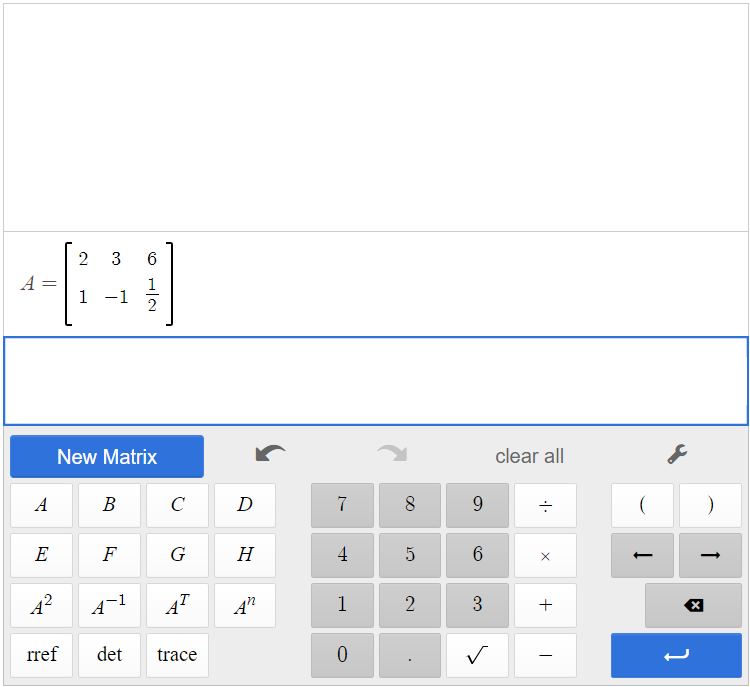
Solve the given system by Gaussian elimination.
[latex]\begin{cases}2x+3y=6\\x-y=\frac{1}{2}\end {cases}[/latex]
First we write this as an augmented matrix.
[latex]\left[ \begin{array}{cc|c} 2&3&6\\1&-1&\frac{1}{2} \end{array} \right ][/latex]
Create matrix A in the calculator by clicking [latex]\begin{array}{|c|}\hline \text{New Matrix}\\ \hline \end{array}\;[/latex]. The augmented matrix is a [latex]2 \times 3[/latex] matrix, so add one column to matrix A, and fill in the entries. Note that the vertical line of the augmented matrix will not be in matrix A in the calculator.
Click [latex]\begin{array}{|c|}\hline \text{rref}\\ \hline \end{array}\;[/latex][latex]\begin{array}{|c|}\hline \text{A}\\ \hline \end{array}\;[/latex], and the calculator will find the row-echelon form of the matrix. By clicking the button next to the solution, you can convert fractions to decimals and decimals to fractions.

Therefore, [latex]\text{rref}(\text{A})=\left[ \begin{array}{cc|c} 1&0& \frac{3}{2}\\0&1&1 \end{array} \right ][/latex]. From the first row, we see that [latex]x=\frac{3}{2}[/latex], and from the second row, we see that [latex]y=1[/latex], making the solution the point [latex](\frac{3}{2}, 1)[/latex].
Use Gaussian elimination to solve the given system of equations.
[latex]\begin{cases}2x+y=1\\4x+2y=6 \end{cases}[/latex]
Write the system as an augmented matrix.
[latex]\left[ \begin{array}{cc|c}2&1&1\\4&2&6 \end{array}\right ][/latex]
Create matrix A in the calculator by clicking [latex]\begin{array}{|c|}\hline \text{New Matrix}\\ \hline \end{array}\;[/latex]. The augmented matrix is a [latex]2 \times 3[/latex] matrix, so add one column to matrix A, and fill in the entries.

Click [latex]\begin{array}{|c|}\hline \text{rref}\\ \hline \end{array}\;[/latex][latex]\begin{array}{|c|}\hline \text{A}\\ \hline \end{array}\;[/latex], and the calculator will find the row-echelon form of the matrix. By clicking the button next to the solution, you can convert fractions to decimals and decimals to fractions.
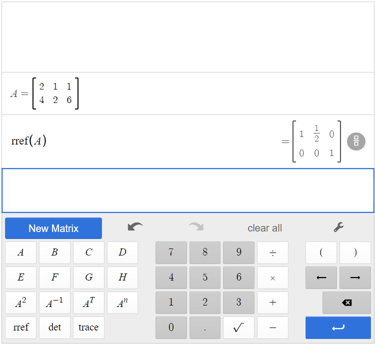
So, [latex]\text{rref}(\text{A})=\left[ \begin{array}{cc|c} 1& \frac{1}{2}&0\\0&0&1 \end{array} \right ][/latex].
The second row represents the equation [latex]0=1[/latex]. Therefore, the system is inconsistent and has no solution.
Solve the system of equations.
[latex]\begin{cases}3x+4y=12\\6x+8y=24\end{cases}[/latex]
Write the system as an augmented matrix.
[latex]\left[ \begin{array}{cc|c}2&1&1\\4&2&6 \end{array}\right ][/latex]
Create matrix A in the calculator by clicking [latex]\begin{array}{|c|}\hline \text{New Matrix}\\ \hline \end{array}\;[/latex]. The augmented matrix is a [latex]2 \times 3[/latex] matrix, so add one column to matrix A, and fill in the entries.
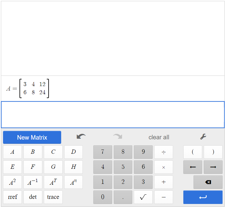
Click [latex]\begin{array}{|c|}\hline \text{rref}\\ \hline \end{array}\;[/latex][latex]\begin{array}{|c|}\hline \text{A}\\ \hline \end{array}\;[/latex], and the calculator will find the row-echelon form of the matrix.
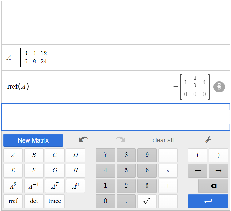
So, [latex]\text{rref}(\text{A})=\left[ \begin{array}{cc|c} 1& \frac{4}{3}&4\\0&0&0 \end{array} \right ][/latex].
The matrix ends up with all zeros in the last row. Thus, there are an infinite number of solutions, and the system is classified as dependent. To find the generic solution, return to one of the original equations and solve for [latex]y[/latex].
[latex]\begin {array}{rcl}3x+4y&=&12\\4y&=&12-3x\\y&=&3-\frac{3}{4}x \end{array}[/latex]
So the solution to this system is [latex](x, 3-\frac{3}{4}x)[/latex].
Solve the system of linear equations using matrices.
[latex]\begin {cases}x-y+z=8\\2x+3y-z=-2\\3x-2y-9z=9\end{cases}[/latex]
First, we write the augmented matrix.
[latex]\left[ \begin{array}{ccc|c}1&-1&1&8\\2&3&-1&-2\\3&-2&-9&9\end{array} \right][/latex]
Create matrix A in the matrix calculator. The size of matrix A is [latex]3 \times 4[/latex].

Click [latex]\begin{array}{|c|}\hline \text{rref}\\ \hline \end{array}\;[/latex][latex]\begin{array}{|c|}\hline \text{A}\\ \hline \end{array}\;[/latex] to find the reduced row-echelon form of matrix A.
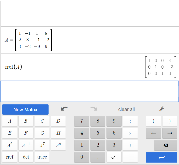
So, [latex]\text{rref}(\text{A})=\left[ \begin{array}{ccc|c}1&0&0&4\\0&1&0&-3\\0&0&1&1\end{array} \right][/latex]. Therefore, the solution to the system is [latex](4, -3, 1)[/latex].
Peter is planning on investing in what’s called a three-fund portfolio, consisting of a U.S. stock mutual fund, an international stock mutual fund, and a bond mutual fund. He has a total of $200,000 to invest and wants four times as much invested in stocks as in bonds. The bond fund has a historical return of 4.4%, the U.S. stock fund has a historical return of 8.3%, and the international stock fund has a historical return of 5.4%. If Peter is hoping for a $13,300 return, how should he allocate his investment?
Of course, historical returns cannot predict future earnings, but they’re the best information we have, so we’ll use them.
We have a system of three equations in three variables.
Let [latex]x[/latex] be the amount invested in U.S. stocks at 8.3% return, and
let [latex]y[/latex] be the amount invested in international stock at 5.4% return.
Let [latex]z[/latex] be the amount invested in the bond fund at 4.4% return.
We have a total of $200,000 to invest, so
[latex]x+y+z=$200,000[/latex]
He wants four times as much invested in stocks as in bonds, so
[latex]\begin{array}{rcl}x+y&=&4z\\x+y-4z&=&0 \end{array}[/latex]
And using the return rates and the desired earnings,
[latex]0.083x+0.054y+0.044z=13,300[/latex]
We can take this system and put it into an augmented matrix.
[latex]A=\left[ \begin{array}{ccc|c}1&1&1&200,000\\1&1&-4&0\\0.083&0.054&0.044&13,300\end{array}\right][/latex]
By plugging matrix A into the calculator and finding the reduced row-echelon form, we get [latex]\text{rref}(\text{A})=\left[ \begin{array}{ccc|c}1&0&0&100,000\\0&1&0&60,000\\0&0&1&40000\end{array}\right][/latex]
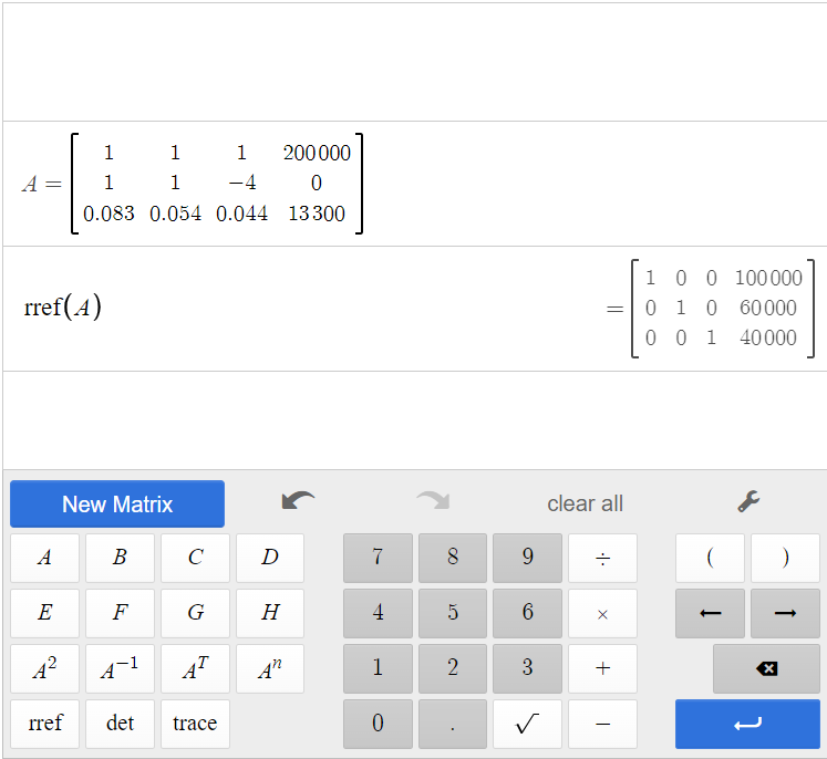
The first row tells us [latex]x=100,000[/latex]. The second row tells us [latex]y=60,000[/latex], and the third row tells us [latex]z=40,000[/latex]. Therefore, $100,000 should be invested in U.S. stock, $60,000 in international stock, and $40,000 in bonds.
Solve the following system of linear equations using matrices.
[latex]\begin{cases}-x-2y+z=-1\\2x+3y=2\\y-2z=0 \end{cases}[/latex]
Write the augmented matrix.
[latex]\left[ \begin{array}{ccc|c}-1&-2&1&-1\\2&3&0&2\\0&1&-2&0\end{array} \right][/latex]
By plugging matrix A into the calculator and finding the reduced row-echelon form, we get [latex]\text{rref}(\text{A})=\left[ \begin{array}{ccc|c}1&0&3&1\\0&1&-2&0\\0&0&0&0\end{array}\right][/latex]
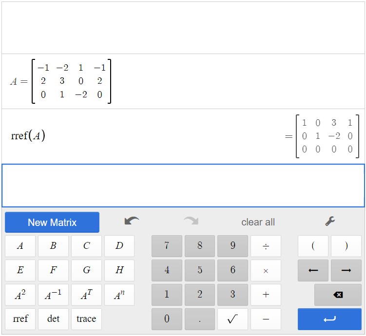
This matrix represents the following system.
[latex]\begin{array}{rcl}x+2y-z&=&1\\y-2z&=&0\\0&=&0 \end{array}[/latex]
We see by the identity [latex]0=0[/latex] that this is a dependent system with an infinite number of solutions. We then find the generic solution. By solving the second equation for [latex]y[/latex] and substituting it into the first equation, we can solve for [latex]z[/latex] in terms of [latex]x[/latex].
[latex]\begin{array}{rcl}x+2y-z&=&1\\y&=&2z\\ \\ x+2(2z)-z&=&1\\x+3z&=&1\\z&=&\frac{1-x}{3} \end{array}[/latex]
Now we substitute the expression for [latex]z[/latex] into the second equation to solve for [latex]y[/latex] in terms of [latex]x[/latex].
[latex]\begin{array}{rcl}y-2z&=&0\\z&=&\frac{1-x}{3}\\ \\y-2(\frac{1-x}{3})&=&0\\y&=&\frac{2-2x}{3}\end{array}[/latex]
The generic solution is [latex](x, \frac{2-2x}{3}, \frac{1-x}{3})[/latex].
Basic Operations
Basic operations were done by hand in Section 2.3. To perform basic operations in the matrix calculator, start by creating two matrices, matrix A and matrix B. After the matrices are created, use the [latex]\begin{array}{|c|}\hline \text{A}\\ \hline \end{array}\;[/latex] and [latex]\begin{array}{|c|}\hline \text{B}\\ \hline \end{array}\;[/latex] buttons along with the operations buttons to simplify the operations. For instance, if you wanted to know [latex]A \times B[/latex], you would first create matrix A and matrix B, then click [latex]\begin{array}{|c|}\hline \text{A}\\ \hline \end{array}\;[/latex][latex]\begin{array}{|c|}\hline \times\\ \hline \end{array}\;[/latex][latex]\begin{array}{|c|}\hline \text{B}\\ \hline \end{array}\;[/latex].
Examples from Section 2.3
Given [latex]A[/latex] and [latex]B[/latex]:
[latex]A=\begin{bmatrix}2&-10&-2\\14&12&10\\4&-2&2\end{bmatrix}[/latex] and [latex]B=\begin{bmatrix}6&10&-2\\0&-12&-4\\-5&2&-2\end{bmatrix}[/latex]
a) Find the sum.
Create matrices A and B in the calculator by clicking [latex]\begin{array}{|c|}\hline \text{New Matrix}\\ \hline \end{array}\;[/latex].

Click [latex]\begin{array}{|c|}\hline \text{A}\\ \hline \end{array}\;[/latex][latex]\begin{array}{|c|}\hline +\\ \hline \end{array}\;[/latex][latex]\begin{array}{|c|}\hline \text{B}\\ \hline \end{array}\;[/latex], and the result is the sum of the two matrices.
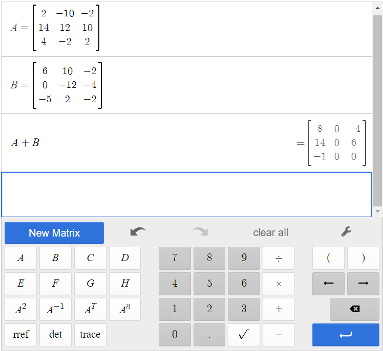
Therefore, [latex]A+B=\begin{bmatrix}8&0&-4\\14&0&6\\-1&0&0\end{bmatrix}[/latex].
b) Find the difference.
Matrices A and B have already been created in the calculator. To find the difference, click [latex]\begin{array}{|c|}\hline \text{A}\\ \hline \end{array}\;[/latex][latex]\begin{array}{|c|}\hline -\\ \hline \end{array}\;[/latex][latex]\begin{array}{|c|}\hline \text{B}\\ \hline \end{array}\;[/latex].
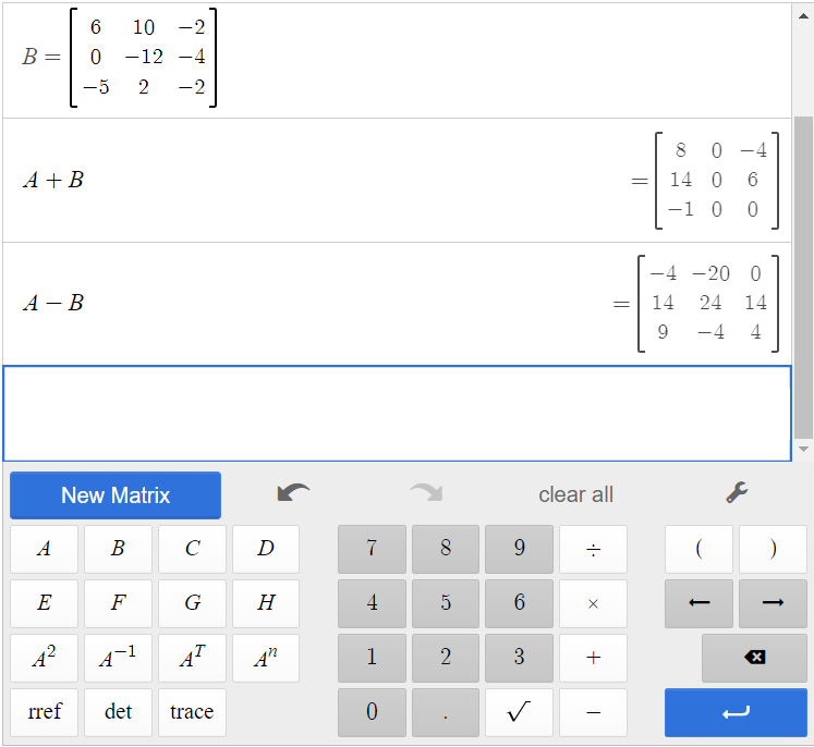
The result is the difference of matrices A and B.
So, [latex]A-B=\begin{bmatrix}-4&-20&0\\14&24&14\\9&-4&4\end{bmatrix}[/latex].
Multiply matrix [latex]A[/latex] by the scalar 3.
[latex]A=\left[\begin{array}{cc}8&1\\5&4 \end{array}\right][/latex]
Create matrix A in the matrix calculator.

Click [latex]\begin{array}{|c|}\hline \text{3}\\ \hline \end{array}\;[/latex][latex]\begin{array}{|c|}\hline \text{A}\\ \hline \end{array}\;[/latex].

Therefore, [latex]3A=\left[\begin{array}{cc}24&3\\15&12\end{array}\right][/latex].
Find the sum [latex]3A+2B[/latex].
[latex]A=\begin{bmatrix}1&-2&0\\0&-1&2\\4&3&-6 \end{bmatrix}[/latex] and [latex]B=\begin{bmatrix}-1&2&1\\0&-3&2\\0&1&-4 \end{bmatrix}[/latex]
Create A and B in the matrix calculator.

Click [latex]\begin{array}{|c|}\hline \text{3}\\ \hline \end{array}\;[/latex][latex]\begin{array}{|c|}\hline \text{A}\\ \hline \end{array}\;[/latex][latex]\begin{array}{|c|}\hline +\\ \hline \end{array}\;[/latex][latex]\begin{array}{|c|}\hline \text{2}\\ \hline \end{array}\;[/latex][latex]\begin{array}{|c|}\hline \text{B}\\ \hline \end{array}\;[/latex].
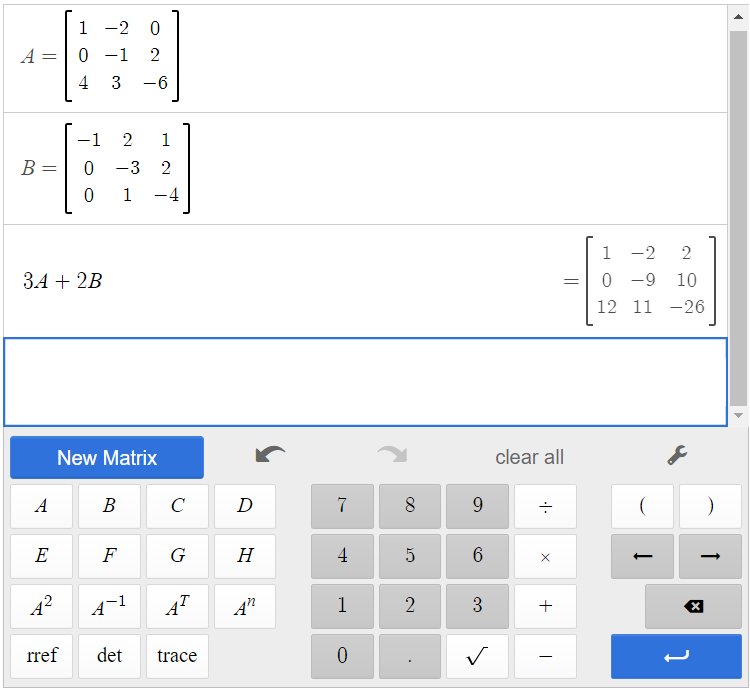
[latex]3A+2B=\begin{bmatrix}1&-2&2\\0&-9&10\\12&11&-26\end{bmatrix}[/latex]
Multiply matrix [latex]A[/latex] and matrix [latex]B.[/latex]
[latex]A=\begin{bmatrix} 1&2\\3&4 \end {bmatrix}[/latex] and [latex]\begin{bmatrix} 5&6\\7&8 \end{bmatrix}[/latex]
First, we check the dimensions of the matrices.
Matrix [latex]A[/latex] has dimensions [latex]2 \times 2[/latex], and matrix [latex]B[/latex] has dimensions [latex]2 \times 2[/latex]. The inner dimensions are the same, so we can perform the multiplication. The product will have the dimensions [latex]2 \times 2[/latex].
Input matrices A and B in the matrix calculator.

Click [latex]\begin{array}{|c|}\hline \text{A}\\ \hline \end{array}\;[/latex][latex]\begin{array}{|c|}\hline \times\\ \hline \end{array}\;[/latex][latex]\begin{array}{|c|}\hline \text{B}\\ \hline \end{array}\;[/latex].
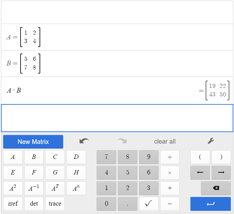
The result is [latex]A \times B =\begin{bmatrix}19&22\\43&50\end{bmatrix}[/latex].
Given [latex]A[/latex] and [latex]B[/latex]:
[latex]A=\begin{bmatrix} -1&2&3\\4&0&5 \end {bmatrix}[/latex] and [latex]B=\begin{bmatrix} 5&-1\\-4&0\\2&3 \end{bmatrix}[/latex]
a) Find [latex]AB[/latex].
As the dimensions of [latex]A[/latex] are [latex]2 \times 3[/latex] and the dimensions of [latex]B[/latex] are [latex]3 \times 2[/latex], these matrices can be multiplied together because the number of columns in [latex]A[/latex] matches the number of rows in [latex]B[/latex]. The resulting product will be a [latex]2 \times 2[/latex] matrix, the number of rows in [latex]A[/latex] by the number of columns in [latex]B[/latex].
Input matrices A and B in the calculator.

Click [latex]\begin{array}{|c|}\hline \text{A}\\ \hline \end{array}\;[/latex][latex]\begin{array}{|c|}\hline \times\\ \hline \end{array}\;[/latex][latex]\begin{array}{|c|}\hline \text{B}\\ \hline \end{array}\;[/latex].
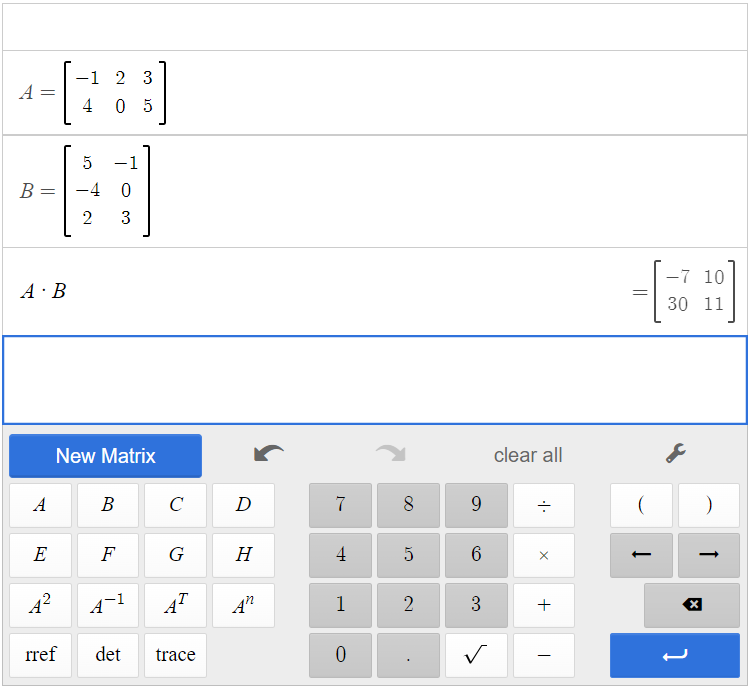
The result is [latex]A \times B =\begin{bmatrix}-7&10\\30&11\end{bmatrix}[/latex].
b) Find [latex]BA[/latex].
The dimensions of [latex]B[/latex] are [latex]3 \times 2[/latex], and the dimensions of [latex]A[/latex] are [latex]2 \times 3[/latex]. The inner dimensions match, so the product is defined and will be a [latex]3 \times 3[/latex] matrix.
Matrices A and B have already been entered into the calculator. Simply click [latex]\begin{array}{|c|}\hline \text{B}\\ \hline \end{array}\;[/latex][latex]\begin{array}{|c|}\hline \times\\ \hline \end{array}\;[/latex][latex]\begin{array}{|c|}\hline \text{A}\\ \hline \end{array}\;[/latex].
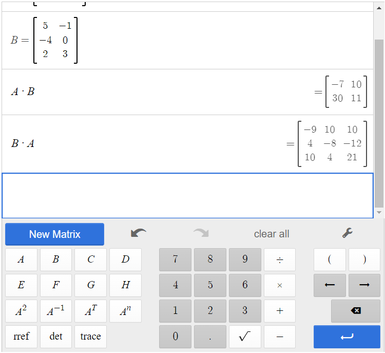
The result is [latex]B \times A =\begin{bmatrix}-9&10&10\\4&-8&-12\\10&4&21\end{bmatrix}[/latex].
Let’s return to the problem presented at the opening of Section 2.3. We have the table below representing the equipment needs of two soccer teams.
[latex]\begin{array}{lcc} &\text{Wildcats}&\text{Mud Cats}\\ \text{Goals}&6&10\\ \text{Balls} &30&24\\ \text{Jerseys}&14&20 \end{array}[/latex]
We are also given the prices of the equipment, as shown below.
[latex]\begin{array}{cc} \text{Goal}& \$300\\ \text{Ball}&$10\\ \text{Jersey}&$30 \end{array}[/latex]
We will convert the data to matrices. Thus, the equipment need matrix is written as
[latex]E=\begin{bmatrix} 6&10\\30&24\\14&20 \end{bmatrix}[/latex]
The cost matrix is written as
[latex]C=\begin{bmatrix} 300&10&30\end{bmatrix}[/latex]
When putting these matrices into the calculator, matrix E was input as matrix A, and matrix C was input as matrix B.
We perform matrix multiplication to obtain costs for the equipment. Due to the dimensions of the matrices, we have to multiply [latex]\begin{array}{|c|}\hline \text{B}\\ \hline \end{array}\;[/latex][latex]\begin{array}{|c|}\hline \times\\ \hline \end{array}\;[/latex][latex]\begin{array}{|c|}\hline \text{A}\\ \hline \end{array}\;[/latex].

The total cost for equipment for the Wildcats is $2,520, and the total cost for equipment for the Mud Cats is $3,840.
Inverses
Inverses were used to solve systems of equations in Section 2.4. To find an inverse in the matrix calculator, start by creating matrix A. Click [latex]\begin{array}{|c|}\hline \text{A}\\ \hline \end{array}\;[/latex] [latex]\begin{array}{|c|}\hline \text{A} ^{-1}\\ \hline \end{array}\;[/latex].
Examples from Section 2.4
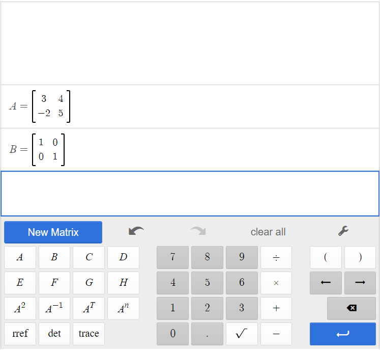
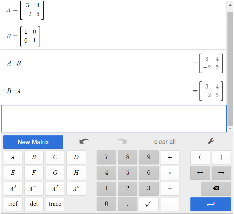
Given matrix [latex]A[/latex], show that [latex]AI=IA=A[/latex].
[latex]A=\begin{bmatrix} 3&4\\-2&5\end{bmatrix}[/latex]
Use matrix multiplication to show that the product of [latex]A[/latex] and the identity is equal to the product of the identity and [latex]A[/latex].
Create matrix A in the calculator, and input matrix A. Then create matrix B in the calculator, and input the identity matrix.
When we type [latex]\begin{array}{|c|}\hline \text{A}\\ \hline \end{array}\;[/latex][latex]\begin{array}{|c|}\hline \times\\ \hline \end{array}\;[/latex][latex]\begin{array}{|c|}\hline \text{B}\\ \hline \end{array}\;[/latex] and [latex]\begin{array}{|c|}\hline \text{B}\\ \hline \end{array}\;[/latex][latex]\begin{array}{|c|}\hline \times\\ \hline \end{array}\;[/latex][latex]\begin{array}{|c|}\hline \text{A}\\ \hline \end{array}\;[/latex], we see that [latex]AI=\begin{bmatrix} 3&4\\-2&5\end{bmatrix}=IA[/latex].
Show that the given matrices are multiplicative inverses of each other.
[latex]A=\begin{bmatrix} 1&5\\-2&-9\end{bmatrix}[/latex], [latex]B=\begin{bmatrix} -9&-5\\2&1\end{bmatrix}[/latex]
Multiply [latex]AB[/latex] and [latex]BA[/latex]. If both products equal the identity, then the two matrices are inverses of each other.

Because [latex]AB=BA=I[/latex], the matrices are inverses of each other.
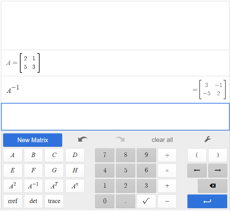
Given [latex]A=\begin{bmatrix}2&1\\5&3\end{bmatrix}[/latex], augment [latex]A[/latex] with the identity [latex]\left[ \begin{array}{cc|cc}2&1&1&0\\5&3&0&1\end{array}\right][/latex]. Find the reduced row-echelon form to turn A into the identity.
Create a new matrix in the calculator that is [latex]2 \times 4[/latex]. We will call this matrix A in the calculator. Let [latex]A=\begin{bmatrix} 2&1&1&0\\5&3&0&1\end{bmatrix}[/latex].
By finding reduced row-echelon form, we can find the inverse of A.

So, [latex]A^{-1} = \begin{bmatrix} 3&-1\\-5&2\end{bmatrix}[/latex].
Use the formula to find the multiplicative inverse of
[latex]A=\begin{bmatrix}2&1\\5&3\end{bmatrix}[/latex]
Using the formula, we have
[latex]\begin{array}{rcl}A^{-1}&=&\frac{1}{(2)(3)-(5)(1)}\begin{bmatrix}3&-1\\-5&2\end{bmatrix}\\ &=&\frac{1}{1}\begin{bmatrix}3&-1\\-5&2\end{bmatrix}\\ &=&\begin{bmatrix}3&-1\\-5&2\end{bmatrix}\\ \end{array}[/latex]
We can also find the inverse without using the formula if we choose to use the matrix calculator. To input the [latex]A^{-1}[/latex] in the calculator, we can input matrix A in the calculator, then click [latex]\begin{array}{|c|}\hline A\\ \hline \end{array}\;[/latex][latex]\begin{array}{|c|}\hline A^{-1}\\ \hline \end{array}\;[/latex].
Notice this matches the inverse we found above by augmenting with the identity matrix.
Find the inverse, if it exists, of the given matrix: [latex]A=\begin{bmatrix} 3&6\\1&2\end{bmatrix}[/latex].
Input the matrix into the matrix calculator, then click [latex]\begin{array}{|c|}\hline A\\ \hline \end{array}\;[/latex][latex]\begin{array}{|c|}\hline A^{-1}\\ \hline \end{array}\;[/latex].
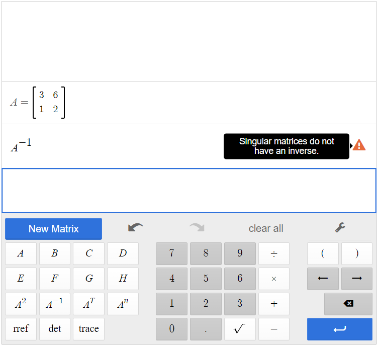
Notice that there is an error when you try to input [latex]A^{-1}[/latex]. This means that there is no inverse of matrix A.
Given the [latex]3\times3[/latex] matrix [latex]A[/latex], find the inverse.
[latex]A=\begin{bmatrix}2&3&1\\3&3&1\\2&4&1\end{bmatrix}[/latex]
Input the matrix into the calculator and click [latex]\begin{array}{|c|}\hline A\\ \hline \end{array}\;[/latex][latex]\begin{array}{|c|}\hline A^{-1}\\ \hline \end{array}\;[/latex].
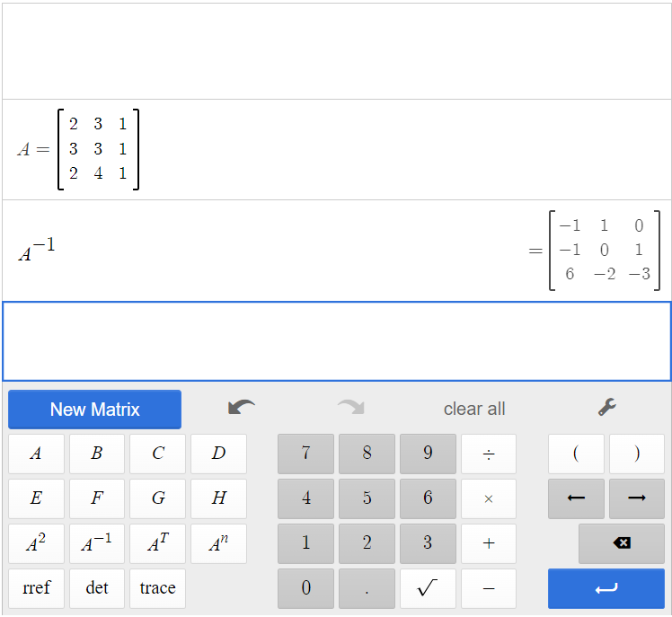
The inverse of matrix A is [latex]A^{-1}=\begin{bmatrix}-1&1&0\\-1&0&1\\6&-3&-2\end{bmatrix}[/latex].
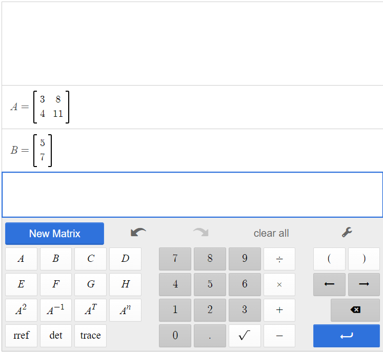
Solve the given system of equations using the inverse of a matrix.
[latex]\begin{cases}3x+8y=5\\4x+11y=7\end {cases}[/latex]
Write the system in terms of a coefficient matrix, a variable matrix, and a constant matrix.
[latex]A=\begin{bmatrix}3&8\\4&11\end{bmatrix}[/latex], [latex]X=\begin{bmatrix}x\\y\end{bmatrix}[/latex], [latex]B=\begin{bmatrix}5\\7\end{bmatrix}[/latex]
Input matrices A and B in the matrix calculator.
Then
[latex]\begin{bmatrix}3&8\\4&11\end{bmatrix}\begin{bmatrix}x\\y\end{bmatrix}=\begin{bmatrix}5\\7\end{bmatrix}[/latex]
First we have to calculate [latex]A^{-1}[/latex].
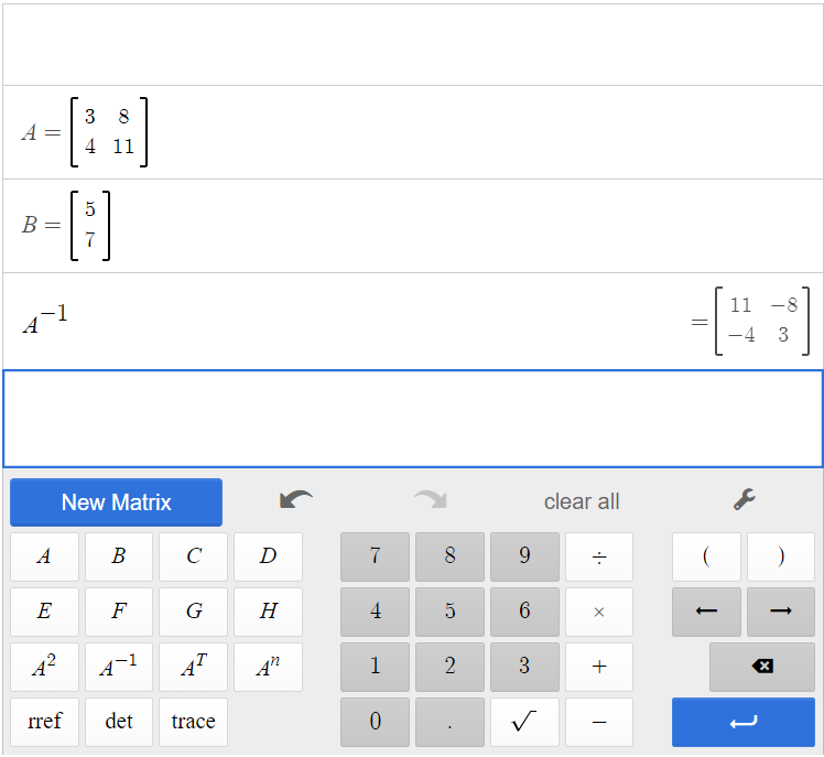
[latex]A^{-1} = \begin{bmatrix}11&8\\-4&3\end{bmatrix}[/latex]
Now we are ready to solve. Multiply both sides of the equation by [latex]A^{-1}[/latex], and use the calculator to simplify all matrix multiplication.
[latex]\begin{array}{rcl}(A^{-1})AX&=&(A^{-1})B\\ \begin{bmatrix}11&-8\\-4&3\end{bmatrix}\begin{bmatrix}3&8\\4&11\end{bmatrix}\begin{bmatrix}x\\y\end{bmatrix}&=&\begin{bmatrix}11&-8\\-4&3\end{bmatrix}\begin{bmatrix}5\\7\end{bmatrix}\\ \begin{bmatrix}1&0\\0&1\end{bmatrix}\begin{bmatrix}x\\y\end{bmatrix}&=&\begin{bmatrix}-1\\1\end{bmatrix}\\ \begin{bmatrix}x\\y\end{bmatrix}&=&\begin{bmatrix}-1\\1\end{bmatrix}\\ \end{array}[/latex].
The solution is [latex](-1,1)[/latex].
Solve the following system using the inverse of a matrix.
[latex]\begin{cases}5x+15y+56z=35\\-4x-11y-41z=-26\\-x-3y-11z=-7\end {cases}[/latex]
Write the equation [latex]AX=B[/latex].
[latex]\begin{bmatrix}5&15&56\\-4&-11&-41\\-1&-3&-11\end{bmatrix}\begin{bmatrix}x\\y\\z\end{bmatrix}=\begin{bmatrix}35\\-26\\-7\end{bmatrix}[/latex]
First, we will find the inverse of [latex]A[/latex] by augmenting with the identity.
[latex]\left[ \begin{array}{ccc|ccc}5&15&56&1&0&0\\-4&-11&-41&0&1&0\\-1&-3&-11&0&0&1\end{array}\right][/latex]
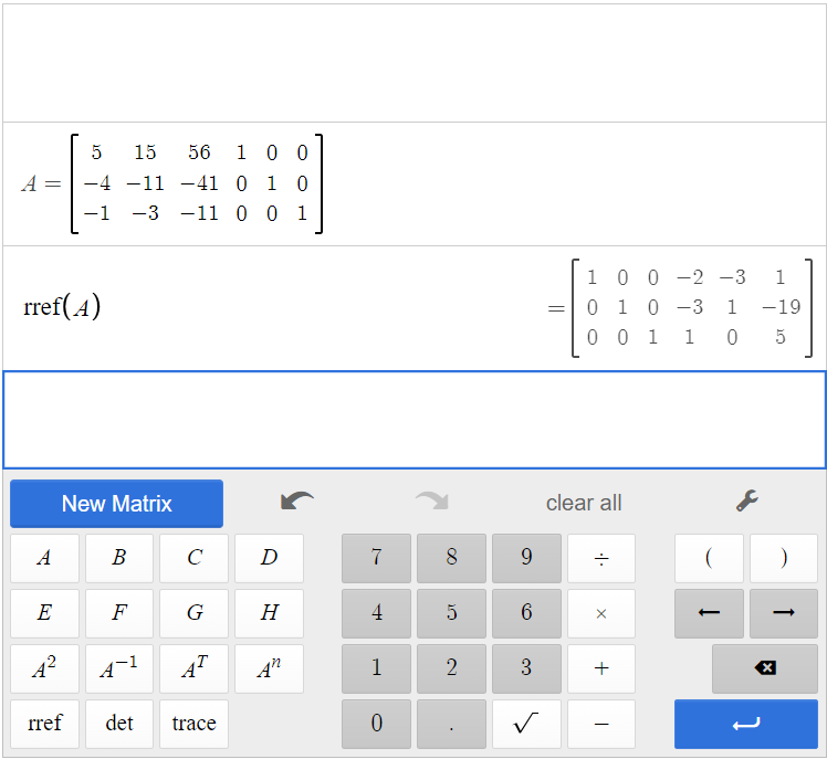
So, [latex]A^{-1}=\begin{bmatrix}-2&-3&1\\-3&1&-19\\1&0&5\end{bmatrix}[/latex].
Multiply both sides of the equation by [latex]A^{-1}[/latex]. We want [latex]A^{-1}AX=A^{-1}B[/latex]:
[latex]\begin{bmatrix}-2&-3&1\\-3&1&-19\\1&0&5\end{bmatrix}\begin{bmatrix}5&15&56\\-4&-11&-41\\-1&-3&-11\end{bmatrix}\begin{bmatrix}x\\y\\z\end{bmatrix}=\begin{bmatrix}-2&-3&1\\-3&1&-19\\1&0&5\end{bmatrix}\begin{bmatrix}35\\-26\\-7\end{bmatrix}[/latex]
Thus,
[latex]A^{-1}B=\begin{bmatrix}1\\2\\0\end{bmatrix}[/latex]
The solution is [latex](1,2,0)[/latex].
Media Attributions
- 2.5 01 is licensed under a CC0 (Creative Commons Zero) license
- 2.5 02 is licensed under a CC0 (Creative Commons Zero) license
- 2.5 05 is licensed under a CC0 (Creative Commons Zero) license
- 2.5 06 is licensed under a CC0 (Creative Commons Zero) license
- 2.5 03 is licensed under a CC0 (Creative Commons Zero) license
- 2.5 04 is licensed under a CC0 (Creative Commons Zero) license
- 2.5 07 is licensed under a CC0 (Creative Commons Zero) license
- 2.5 08 is licensed under a CC0 (Creative Commons Zero) license
- 2.5 09 is licensed under a CC0 (Creative Commons Zero) license
- 2.5 10 is licensed under a CC0 (Creative Commons Zero) license
- 2.5 11 is licensed under a CC0 (Creative Commons Zero) license
- 2.5 12 is licensed under a CC0 (Creative Commons Zero) license
- 2.5 13 is licensed under a CC0 (Creative Commons Zero) license
- 2.5 14 is licensed under a CC0 (Creative Commons Zero) license
- 2.5 15 is licensed under a CC0 (Creative Commons Zero) license
- 2.5 16 is licensed under a CC0 (Creative Commons Zero) license
- 2.5 17 is licensed under a CC0 (Creative Commons Zero) license
- 2.5 18 is licensed under a CC0 (Creative Commons Zero) license
- 2.5 19 is licensed under a CC0 (Creative Commons Zero) license
- 2.5 20 is licensed under a CC0 (Creative Commons Zero) license
- 2.5 21 is licensed under a CC0 (Creative Commons Zero) license
- 2.5 22 is licensed under a CC0 (Creative Commons Zero) license
- 2.5 23 is licensed under a CC0 (Creative Commons Zero) license
- 2.5 24 is licensed under a CC0 (Creative Commons Zero) license
- 2.5 25 is licensed under a CC0 (Creative Commons Zero) license
- 2.5 26 is licensed under a CC0 (Creative Commons Zero) license
- 2.5 27 is licensed under a CC0 (Creative Commons Zero) license
- 2.5 28 is licensed under a CC0 (Creative Commons Zero) license
- 2.5 29 is licensed under a CC0 (Creative Commons Zero) license
- 2.5 30 is licensed under a CC0 (Creative Commons Zero) license
- 2.5 31 is licensed under a CC0 (Creative Commons Zero) license
- 2.5 32 is licensed under a CC0 (Creative Commons Zero) license
- 2.5 33 is licensed under a CC0 (Creative Commons Zero) license
- 2.5 34 is licensed under a CC0 (Creative Commons Zero) license
