Chapter 2 Matrices
2.2 Solving Systems Using Matrices
Learning Objectives
By the end of this section, you will be able to:
- Write a system of equations as an augmented matrix.
- Use a matrix and row-reduction (Gaussian elimination) to solve a system of equations.
- Interpret the solutions from an augmented matrix.
- Recognize dependent and inconsistent systems of equations.
While the techniques we learned in the last section can be used to solve any 2-by-2 or 3-by-3 system of linear equations, mathematicians often look for ways to do problems while writing less (which is why we use single letters for variables instead of full words), and to make solving problems more procedural. For systems of linear equations, matrices are the tool we use. In addition to making solving small systems more straightforward, the techniques can be extended to solve 4-by-4, 100-by-100, or even larger systems of linear equations that common arise in science.
A matrix is a rectangular array of numbers arranged into rows and columns.
Writing the Augmented Matrix of a System of Equations
A matrix can serve as a device for representing and solving a system of equations. To express a system in matrix form, we extract the coefficients of the variables and the constants, and these become the entries of the matrix. We use a vertical line to separate the coefficient entries from the constants, essentially replacing the equal signs. When a system is written in this form, we call it an augmented matrix.
Given a system of equations, write an augmented matrix:
- Write the coefficients of the x-terms as the numbers down the first column.
- Write the coefficients of the y-terms as the numbers down the second column.
- If there are z-terms, write the coefficients as the numbers down the third column.
- Draw a vertical line and write the constants to the right of the line.
Example 1
Consider the following 2×2 system of equations. Write this system as an augmented matrix:
[latex]\begin{cases}3x+4y=7\\4x-2y=5\end {cases}[/latex]
Extracting the coefficients from the system and write them in a rectangular array. This is called the coefficient matrix.
[latex]\begin{bmatrix}3&4\\4&-2\end{bmatrix}[/latex]
We then draw a vertical line and extract the constants from the right hand side of the system equations. This is the augmented matrix for the given system.
[latex]\left[ \begin{array}{cc|c}3&4&7\\4&-2&5\end{array}\right][/latex]
Example 2
Write the augmented matrix for the three-by-three system of equations.
[latex]\begin{cases}3x-y-z=0\\x+y=5\\2x-3z=2\end{cases}[/latex]
The coefficient matrix is
[latex]\begin{bmatrix}3&-1&-1\\1&1&0\\2&0&-3\end{bmatrix}[/latex]
And the system is represented by the augmented matrix
[latex]\left[ \begin{array}{ccc|c}3&-1&-1&0\\1&1&0&5\\2&0&-3&2\end{array}\right][/latex]
Notice that the matrix is written so that the variables line up in their own columns: [latex]x[/latex]-terms go in the first column, [latex]y[/latex]-terms in the second column, and [latex]z[/latex]-terms in the third column. It is very important that each equation is written in standard form so that the variables line up. When there is a missing variable term in an equation, the coefficient is 0.
Exercise 1
Write the augmented matrix of the given system of equations.
[latex]\begin{cases}4x-3y=11\\3x+2y=4\end{cases}[/latex]
Solution
[latex]\left[ \begin{array}{cc|c}4&-3&11\\3&2&4\end{array}\right][/latex]
Writing a System of Equations from an Augmented Matrix
We can use augmented matrices to help us solve systems of equations because they simplify operations when the systems are not encumbered by the variables. However, it is important to understand how to move back and forth between formats in order to make finding solutions smoother and more intuitive. Here, we will use the information in an augmented matrix to write the system of equations in standard form.
Example 3
Find the system of equations from the augmented matrix.
[latex]\left[ \begin{array}{ccc|c}1&-3&-5&-2\\2&-5&-4&5\\-3&5&4&6\end{array}\right][/latex]
When the columns represent the variables [latex]x[/latex], [latex]y[/latex], and [latex]z[/latex],
[latex]\left[ \begin{array}{ccc|c}1&-3&-5&-2\\2&-5&-4&5\\-3&5&4&6\end{array}\right]\rightarrow\begin{array}{rcl}x-3y-5z&=&-2\\2x-5y-4z&=&5\\-3x+5y+4z&=&6\end{array}[/latex]
Exercise 2
Write the system of equations from the augmented matrix.
[latex]\left[ \begin{array}{ccc|c}1&-1&1&5\\2&-1&3&1\\0&1&1&-9\end{array}\right][/latex]
Solution
[latex]\begin{array}{rcl}x-y+z&=&5\\2x-y+3z&=&1\\y+z&=&-9\end{array}[/latex]
Performing Row Operations on a Matrix
Now that we can write systems of equations in augmented matrix form, we will examine the various row operations that can be performed on a matrix, such as addition, multiplication by a constant, and interchanging rows. These are all operations that can be performed without changing the solution to the corresponding system.
Performing row operations on a matrix is the method we use for solving a system of equations, since these operations allow us to change a complex system into an equivalent simpler one with the same solution. In order to solve the system of equations, we want to convert the matrix to row-echelon form, in which there are ones down the main diagonal from the upper left corner to the lower right corner, and zeros in every position below the main diagonal as shown.
[latex]\text{Row-echelon form}\\ \begin{bmatrix}1&a&b\\0&1&d\\0&0&1\end{bmatrix}[/latex]
We use row operations corresponding to equation operations to obtain a new matrix that is row-equivalent in a simpler form.
Guidelines for row-echelon form:
- In any nonzero row, the first nonzero number is a 1. It is called a leading 1.
- Any all-zero rows are placed at the bottom on the matrix.
- Any leading 1 is below and to the right of a previous leading 1.
- Any column containing a leading 1 has zeros in all other positions in the column.
Solving a system of equations using row operations
To solve a system of equations we can perform the following row operations to convert the coefficient matrix to row-echelon form and do back-substitution to find the solution.
- Interchange rows. (Notation: [latex]R_i\longleftrightarrow R_j[/latex])
- Multiply a row by a constant. (Notation: [latex]cR_i[/latex])
- Add the product of a row multiplied by a constant to another row. (Notation: [latex]R_i+cR_j[/latex])
Each of the row operations corresponds to the operations we have already learned to solve systems of equations in three variables. With these operations, there are some key moves that will quickly achieve the goal of writing a matrix in row-echelon form. To obtain a matrix in row-echelon form for finding solutions, we use Gaussian elimination, a method that uses row operations to obtain a 1 as the first entry so that row 1 can be used to convert the remaining rows.
Gaussian Elimination
The Gaussian elimination method refers to a strategy used to obtain the row-echelon form of a matrix. The goal is to write matrix with the number 1 as the entry down the main diagonal and have all zeros below.
The first step of the Gaussian strategy includes obtaining a 1 as the first entry, so that row 1 may be used to alter the rows below.
[latex]A=\begin{bmatrix}a_{11}&a_{12}&a_{13}\\a_{21}&a_{22}&a_{23}\\a_{31}&a_{32}&a_{33}\end{bmatrix} \xrightarrow[ ]{ \text {After Gaussian elimination }} A=\begin{bmatrix}1&b_{12}&b_{13}\\0&1&b_{23}\\0&0&1\end{bmatrix}[/latex]
Using row operations on an augmented matrix to achieve row-echelon form.
- The first equation should have a leading coefficient of 1. Interchange rows or multiply by a constant, if necessary.
- Use row operations to obtain zeros down the first column below the first entry of 1.
- Use row operations to obtain a 1 in row 2, column 2.
- Use row operations to obtain zeros down column 2, below the entry of 1.
- Use row operations to obtain a 1 in row 3, column 3.
- Continue this process for all rows until there is a 1 in every entry down the main diagonal and there are only zeros below.
- If any rows contain all zeros, place them at the bottom.
Example 4
Solve the given system by Gaussian elimination.
[latex]\begin{cases}2x+3y=6\\x-y=\frac{1}{2}\end {cases}[/latex]
First we write this as an augmented matrix.
[latex]\left[ \begin{array}{cc|c} 2&3&6\\1&-1&\frac{1}{2} \end{array} \right ][/latex]
We want a 1 in row 1, column 1. This can be accomplished by interchanging row 1 and row 2.
[latex]R_1\leftrightarrow R_2 \longrightarrow \left[ \begin{array}{cc|c}1&-1&\frac{1}{2}\\2&3&6\end{array} \right][/latex]
We now have a 1 as the first entry in row 1, column 1. Now let’s obtain a 0 in row 2, column 1. This can be accomplished by multiplying row 1 by -2 and then adding the result to row 2.
[latex]-2R_1+R_2=R_2 \longrightarrow \left[ \begin{array}{cc|c}1&-1&\frac{1}{2}\\0&5&5 \end{array} \right][/latex]
We only have one more step, to multiply row 2 by [latex]\frac{1}{5}[/latex].
[latex]\frac{1}{5}R_2=R_2 \longrightarrow \left[ \begin{array}{cc|c}1&-1&\frac{1}{2}\\0&1&1 \end{array} \right][/latex]
Use back-substitution. The second row of the matrix represents [latex]y=1[/latex]. Back-substitute [latex]y=1[/latex] into the first equation.
[latex]\begin {array}{rcl}x-(1)&=&\frac{1}{2}\\x&=&\frac{3}{2} \end{array}[/latex]
The solution is the point [latex](\frac{3}{2}, 1)[/latex].
Use Gaussian elimination to solve the given system of equations.
[latex]\begin{cases}2x+y=1\\4x+2y=6 \end{cases}[/latex]
Write the system as an augmented matrix.
[latex]\left[ \begin{array}{cc|c}2&1&1\\4&2&6 \end{array}\right ][/latex]
Obtain a 1 in row 1, column 1. This can be accomplished by multiplying the first row by [latex]\frac{1}{2}[/latex]
[latex]\frac{1}{2}R_1=R_1 \longrightarrow \left[ \begin{array}{cc|c}1&\frac{1}{2}&\frac{1}{2}\\4&2&6 \end{array} \right][/latex]
Next, we want a 0 in row 2, column 1. Multiply row 1 by -4 and add row 1 to row 2.
[latex]-4R_1+R_2=R_2\longrightarrow \left[ \begin{array}{cc|c}1&\frac{1}{2}&\frac{1}{2}\\0&0&4 \end{array} \right][/latex]
The second row represents the equation [latex]0=4[/latex]. Therefore, the system is inconsistent and has no solution.
Solve the system of equations.
[latex]\begin{cases}3x+4y=12\\6x+8y=24\end{cases}[/latex]
Perform row operations on the augmented matrix to try and achieve row-echelon form.
[latex]A=\left[ \begin{array}{cc|c}3&4&12\\6&8&24\end{array} \right][/latex]
[latex]\frac{1}{2}R_2+R_1 \longrightarrow \left[ \begin{array}{cc|c}0&0&0\\6&8&24 \end{array} \right][/latex]
[latex]R_1\longleftrightarrow R_2 \longrightarrow \left[ \begin{array}{cc|c}6&8&24\\0&0&0 \end{array}\right][/latex]
The matrix ends up with all zeros in the last row: Thus, there are an infinite number of solutions and the system is classified as dependent. To find the generic solution, return to one of the original equations and solve for [latex]y[/latex].
[latex]\begin {array}{rcl}3x+4y&=&12\\4y&=&12-3x\\y&=&3-\frac{3}{4}x \end{array}[/latex]
So the solution to this system is [latex](x, 3-\frac{3}{4}x)[/latex].
Row reduction can be applied to any size system.
Example 7
Perform row operations on the given matrix to obtain row-echelon form.
[latex]\left[\begin{array}{ccc|c}1&-3&4&3\\2&-5&6&6\\-3&3&4&3\end{array}\right][/latex]
The first row already has a 1 in row 1, column 1. The next step is to multiply row 1 by -2 and add it to row 2. Then replace row 2 with the result.
[latex]-R_1+R_2=R_2 \longrightarrow \left[ \begin{array}{ccc|c}1&-3&4&3\\0&1&-2&0\\-3&3&4&6\end{array} \right][/latex]
Next, obtain a zero in row 3, column 1.
[latex]3R_1+R_3=R_3 \longrightarrow \left[ \begin{array}{ccc|c}1&-3&4&3\\0&1&-2&0\\0&-6&16&15 \end{array}\right][/latex]
Next, obtain a zero in row 3, column 2.
[latex]6R_2+R_3=R_3 \longrightarrow \left[ \begin{array}{ccc|c} 1&-3&4&3\\0&1&-2&0\\0&0&4&15 \end{array} \right][/latex]
The last step is to obtain a 1 in row 3, column 3.
[latex]\frac{1}{2}R_3=R_3 \longrightarrow \left[ \begin{array}{ccc|c}1&-3&4&3\\0&1&-2&-6\\0&0&1&\frac{21}{2}\end{array} \right][/latex]
Exercise 4
Write the system of equations as an augmented matrix, then perform row operations to obtain row-echelon form.
[latex]\begin {cases} x-2y+3z=9\\-x+3y=-4\\2x-5y+5z=17 \end{cases}[/latex]
Solution
[latex]\left[ \begin{array}{ccc|c}1&-\frac{5}{2}&\frac{5}{2}&\frac{17}{2}\\0&1&5&9\\0&0&1&2 \end{array} \right][/latex]
Solving a 3-by-3 System of Linear Equations Using Matrices
We have seen how to write a system of equations with an augmented matrix, and then how to use row operations and back-substitution to obtain row-echelon form. Now, we will take row-echelon form a step farther to solve a 3 by 3 system of linear equations. The general idea is to eliminate all but one variable using row operations and then back-substitute to solve for the other variables.
Example 8
Solve the system of linear equations using matrices.
[latex]\begin {cases}x-y+z=8\\2x+3y-z=-2\\3x-2y-9z=9\end{cases}[/latex]
First, we write the augmented matrix.
[latex]\left[ \begin{array}{ccc|c}1&-1&1&8\\2&3&-1&-2\\3&-2&-9&9\end{array} \right][/latex]
Next, we perform row operations to obtain row-echelon form.
[latex]-2R_1+R_2=R_2 \longrightarrow \left[ \begin{array}{ccc|c}1&-1&1&8\\0&5&-3&-18\\3&-2&-9&9\end{array} \right][/latex]
[latex]-3R_1+R_3=R_3 \longrightarrow \left[ \begin{array}{ccc|c}1&-1&1&8\\0&5&-3&-18\\0&1&-12&-15 \end{array} \right][/latex]
The easiest way to obtain a 1 in row 2 of column 1 is to interchange [latex]R_2[/latex] and [latex]R_3[/latex].
Interchange [latex]R_2[/latex] and [latex]R_3\longrightarrow \left[ \begin{array}{ccc|c}1&-1&1&8\\0&1&-12&-15\\0&5&-3&-18\end{array} \right][/latex]
Then
[latex]-5R_2+R_3=R_3 \longrightarrow \left[ \begin{array}{ccc|c}1&-1&1&8\\0&1&-12&-15\\0&057&57 \end{array}\right][/latex]
[latex]\frac{1}{57}R_3=R_3 \longrightarrow \left[ \begin{array}{ccc|c}1&-1&1&8\\0&1&-12&-15\\0&0&1&1\end{array} \right][/latex]
The last matrix represents the equivalent system.
[latex]\begin{array}{rcl}x-y+z&=&8\\y-12z&=&-15\\z&=&1 \end{array}[/latex]
Using back-substitution, we obtain the solution as [latex](4, -3, 1)[/latex].
Using these approaches, a system of linear equations of any size can be solved by Gaussian elimination. One of the real benefits of Gaussian elimination is that it is very procedural, so it is something we can teach a computer or calculator to do.
Example 9
Peter is planning on investing in what’s called a three fund portfolio, consisting of a U.S. stock mutual fund, an international stock mutual fund, and a bond mutual fund. He has a total of $200,000 to invest, and wants four times as much invested in stocks as in bonds. The bond fund has a historical return of 4.4%, the U.S. stock fund has a historical return of 8.3%, and the international stock fund has a historical return of 5.4%. If Peter is hoping for a $13,300 return, how should he allocate his investment?
Of course, historical returns cannot predict future earnings, but they’re the best information we have, so we’ll use them.
We have a system of three equations in three variables.
let [latex]x[/latex] be the amount invested in U.S. stocks at 8.3% return, and
let [latex]y[/latex] be the amount invested in international stock at 5.4% return.
Let [latex]z[/latex] be the amount invested in the bond fund at 4.4% return,
We have a total of $200,000 to invest, so
[latex]x+y+z=$200,000[/latex]
He wants four times as much invested in stocks as in bonds, so
[latex]\begin{array}{rcl}x+y&=&4z\\x+y-4z&=&0 \end{array}[/latex]
And using the return rates and the desired earnings,
[latex]0.083x+0.054y+0.044z=13,300[/latex]
We can take this system and put it into an augmented matrix.
[latex]\left[ \begin{array}{ccc|c}1&1&1&200,000\\1&1&-4&0\\0.083&0.054&0.044&13,300\end{array}\right][/latex]
Now, we perform Gaussian elimination to achieve row-echelon form.
[latex]-R_1+R_2=R_2\longrightarrow \left[ \begin{array}{ccc|c}1&1&1&200,000\\0&0&-5&-200,000\\0.083&0.054&0.044&13,300\end{array} \right][/latex]
[latex]-0.083R_1+R_3=R_3\longrightarrow \left[ \begin{array}{ccc|c}1&1&1&200,000\\0&0&-5&-200,000\\0&-0.029&-0.039&-3,300\end{array} \right][/latex]
[latex]R_2\leftrightarrow R_3 \longrightarrow \left[ \begin{array}{ccc|c}1&1&1&200,000\\0&-0.029&-0.039&-3,300\\0&0&-5&-200,000\end{array} \right][/latex]
[latex]\frac{1}{-0.029}R_2=R_2\longrightarrow \left[ \begin{array}{ccc|c}1&1&1&200,000\\0&1&\frac{39}{29}&\frac{3,300,000}{29}\\0&0&-5&-200,000\end{array}\right][/latex]
[latex]\frac{1}{-5}R_3=R_3\longrightarrow\left[ \begin{array}{ccc|c}1&1&1&200,000\\0&1&\frac{39}{29}&\frac{3,300,000}{29}\\0&0&1&40,000 \end{array} \right][/latex]
The third row tells us [latex]z=40,000[/latex].
The second row tells us [latex]y+\frac{39}{29}=\frac{3,300,000}{29}[/latex], or [latex]29y+39z=3,300,000[/latex] .
Substituting [latex]z=40,000[/latex] we get
[latex]\begin{array}{rcl}29y+39(40,000)&=&3,300,000\\29y+1,560,000&=&3,300,000\\29y&=&1,740,000\\y&=&60,000\end{array}[/latex]
The first row tells us [latex]x+y+z=200,000[/latex] . Substituting [latex]y=60,000[/latex] and [latex]z=40,000[/latex] we get
[latex]\begin{array}{rcl}x+60,000+40,000&=&200,000\\x&=&100,000\end{array}[/latex]
The answer is $100,000 invested in U.S. stock, $60,000 in international stock, and $40,000 in bonds.
Number of Possible Solutions
Definitions to know:
With three-by-three systems, the possibilities for number of solutions are:
(1) Systems that have a single solution are those which, after elimination, result in a solution set consisting of an ordered triple . Graphically, the ordered triple defines a point that is the intersection of three planes in space.

(2) Systems that have an infinite number of solutions are those which, after Gaussian elimination, have a row of all zeros, equivalent to the statement 0 = 0. Graphically, an infinite number of solutions represents a line or coincident plane that serves as the intersection of three planes in space.
(3) Systems that have no solution are those that, after Gaussian elimination, have a row of all zeros in the coefficient matrix and a nonzero-entry on the right hand side, equivalent to a statement such as Graphically, a system with no solution is represented by three planes with no point in common. There are several ways this can happen, as shown below.
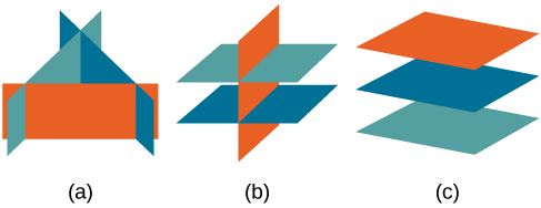
All three figures represent three-by-three systems with no solution. (a) The three planes intersect with each other, but not at a common point. (b) Two of the planes are parallel and intersect with the third plane, but not with each other. (c) All three planes are parallel, so there is no point of intersection
Example 10
Solve the following system of linear equations using matrices.
[latex]\begin{cases}-x-2y+z=-1\\2x+3y=2\\y-2z=0 \end{cases}[/latex]
Write the augmented matrix.
[latex]\left[ \begin{array}{ccc|c}-1&-2&1&-1\\2&3&0&2\\0&1&-2&0\end{array} \right][/latex]
First, multiply row 1 by -1 to get a 1 in row 1, column 1. Then, perform row operations to obtain row-echelon form.
[latex]-R_1\longrightarrow \left[ \begin{array}{ccc|c} 1&2&-1&1\\2&3&0&2\\0&1&-2&0\end{array} \right][/latex]
[latex]R_2\leftrightarrow R_3=R_3\longrightarrow\left[ \begin{array}{ccc|c} 1&2&-1&1\\0&1&-2&0\\2&3&0&2\end{array} \right][/latex]
[latex]-2R_1+R_3=R_3\longrightarrow \left[\begin{array}{ccc|c} 1&2&-1&1\\0&1&-2&0\\0&-1&2&0\end{array} \right][/latex]
[latex]R_2+R_3=R_3\longrightarrow \left[\begin{array}{ccc|c} 1&2&-1&1\\0&1&-2&0\\0&-1&2&0\end{array} \right][/latex]
[latex]R_2+R_3=R_3\longrightarrow\left[ \begin{array}{ccc|c} 1&2&-1&1\\0&1&-2&0\\0&0&0&0\end{array} \right][/latex]
The last matrix represents the following system.
[latex]\begin{array}{rcl}x+2y-z&=&1\\y-2z&=&0\\0&=&0 \end{array}[/latex]
We see by the identity [latex]0=0[/latex] that this is a dependent system with an infinite number of solutions. We then find the generic solution. By solving the second equation for [latex]y[/latex] and substituting it into the first equation we can solve for [latex]z[/latex] in terms of [latex]x[/latex].
[latex]\begin{array}{rcl}x+2y-z&=&1\\y&=&2z\\ \\ x+2(2z)-z&=&1\\x+3z&=&1\\z&=&\frac{1-x}{3} \end{array}[/latex]
Now we substitute the expression for [latex]z[/latex] into the second equation to solve for [latex]y[/latex] in terms of [latex]x[/latex].
[latex]\begin{array}{rcl}y-2z&=&0\\z&=&\frac{1-x}{3}\\ \\y-2(\frac{1-x}{3})&=&0\\y&=&\frac{2-2x}{3}\end{array}[/latex]
The generic solution is [latex](x, \frac{2-2x}{3}, \frac{1-x}{3})[/latex]
Media Attributions
- 2.2 01 © Business Precalculus by David Lippman is licensed under a CC BY-SA (Attribution ShareAlike) license
- 2.2 02 © Business Precalculus by David Lippman is licensed under a CC BY-SA (Attribution ShareAlike) license
- 2.2 03 © Business Precalculus by David Lippman is licensed under a CC BY-SA (Attribution ShareAlike) license
A matrix is a rectangular array of numbers arranged into rows and columns.
A matrix in which we use a vertical line to separate the coefficient entries from the constants, essentially replacing the equal signs.
A matrix formed by extracting the coefficients from the system and writing them in a rectangular array
These are all operations that can be performed on a matrix without changing the solution to the corresponding system. These operations include, addition, multiplication, and interchanging rows.
A matrix form in which there are ones down the main diagonal and zeros in every position below the main diagonal.
The matrix entries that lie on the diagonal from the upper left corner to the lower right corner of a matrix.
Matrices that can be changed from one to another by employing a sequence of row operations.
Gaussian elimination method refers to a strategy used to obtain the row-echelon form of a matrix.
A dependent system is a consistent system whose equations have the same slope and the same y-intercepts.
A system of equations in which the equations represent two parallel lines; hence, there is no solution to the system.
