Chapter 8 Statistics
8.8 Statistics Calculator
Learning Objectives
By the end of this section, you will be able to:
- Use technology to find the following:
- Mean
- Standard deviation
- Five-number summary
- Use technology to plot a histogram
Calculators are useful tools in analyzing large sets of data. Calculators like the Desmos statistics calculator can be used to find important information such as the mean, median, standard deviation, and the five-number summary of any dataset. You can find the Desmos statistics calculator in the link above or in the Back Matter of this book.
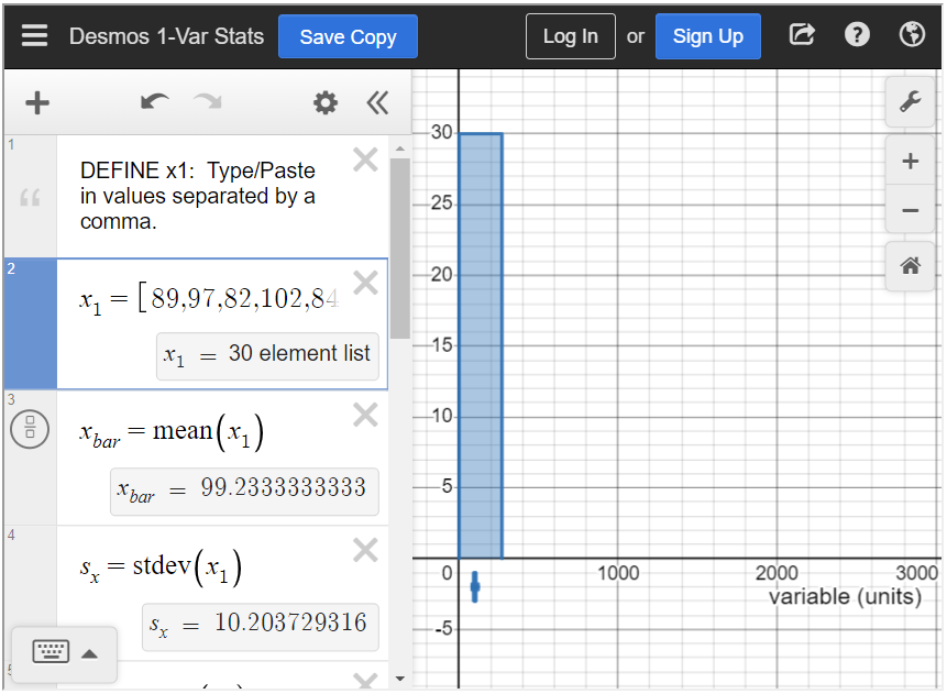
To use the statistics calculator, first input the data values into [latex]x_1 = [\text{ }][/latex], where data values are separated by a comma. After the data are entered, the calculator will give the following data analytics:
- The mean can be found in [latex]x_{bar}=\text{mean(}x_1 \text{)}[/latex].
- The standard deviation can be found in [latex]s_x = \text{stdev(} x_1 \text{)}[/latex].
- The number of elements are given in [latex]n = \text{length(} x_1 \text{)}[/latex].
- The five-number summary can be found in [latex]\text{stats(} x_1 \text{)}[/latex].
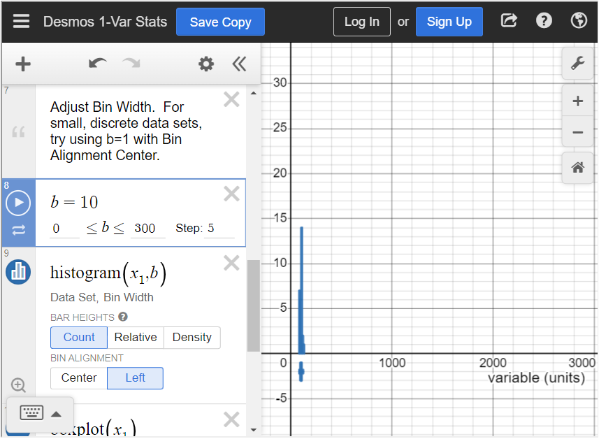
When plotting a histogram, there are some settings that will have to be adjusted. Use [latex]b = 270[/latex] to adjust the bin width of the histogram. You can use the sliding bar or enter a number other than 270. The wrench in the top right corner can be used to adjust additional settings of the histogram. We will explore these settings in Example 7 from Section 8.2.
Examples from Section 8.2
In Example 6, we built a stem-and-leaf plot for the number of chirps made by crickets in one minute. Here are the raw data that we used then:
| 89 | 97 | 82 | 102 | 84 | 99 |
| 115 | 105 | 89 | 109 | 107 | 89 |
| 101 | 109 | 116 | 103 | 100 | 91 |
| 93 | 103 | 120 | 91 | 85 | 104 |
| 104 | 82 | 106 | 92 | 104 | 106 |
Construct a histogram to visualize these results.
Input the data values into the brackets of [latex]x_1[/latex], separated by a comma. As you input the values, you will notice that a histogram will start to form.
We need to adjust the bin setting so that the bars are an appropriate width. Scroll down until you see b = 270. Adjust that to b = 10.
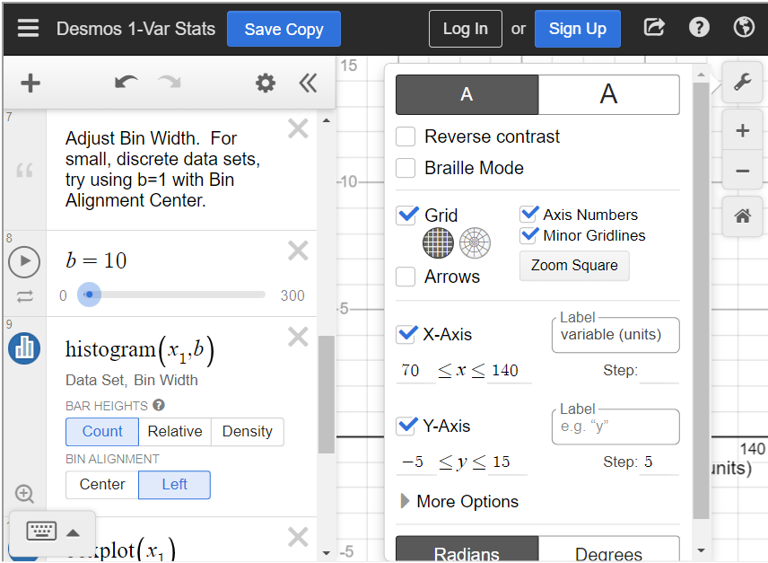
In order to see the histogram, we have to adjust the settings. Click on the wrench in the top right corner to adjust the graph settings. Change the X-Axis settings to [latex]70 \leq x \leq 140[/latex] because all data values are between 70 and 140. Change the Y-Axis settings to [latex]-5 \leq y \leq 15[/latex] because the highest frequency is 14. You can choose different settings if you’d like, but these settings allow us to see the entire histogram.
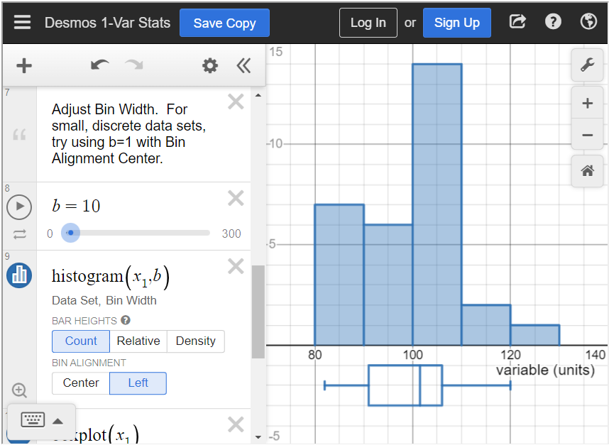
When you close the settings, you can see the histogram.
Examples and Exercises from Section 8.3
In a previous example, we looked at a stem-and-leaf plot that contained 33 sale prices (in dollars) of a particular collectible trading card:
| 0 | 5 8 9 |
| 1 | 0 0 0 3 4 4 5 5 5 5 6 9 9 |
| 2 | 0 0 0 0 5 5 9 9 |
| 3 | 0 0 0 5 5 |
| 4 | 0 0 5 |
| 5 | |
| 6 | 0 |
What is the median price?
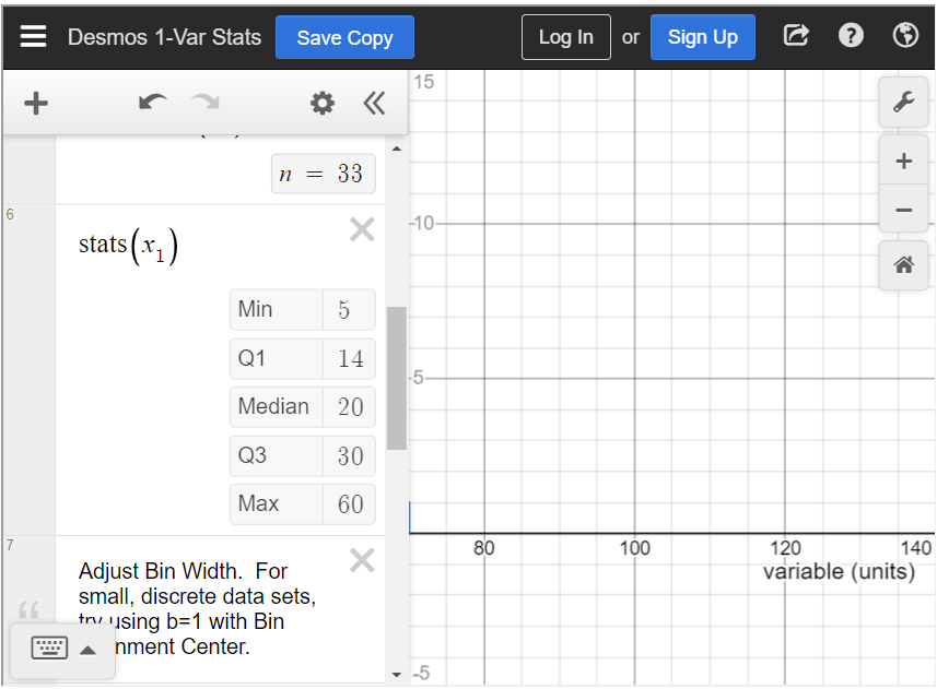
To find the median in the statistics calculator, type all values into [latex]x_1[/latex], separated by a comma. Scroll down until you see “[latex]\text{stats}(x_1)[/latex].” This is the five-number summary of the data. In this table, you can see that the median is 20.
We previously looked at the number of times different crickets (of differing species, genders, etc.) chirped in a one-minute span. Those data are again provided below:
| 89 | 97 | 82 | 102 | 84 | 99 |
| 115 | 105 | 89 | 109 | 107 | 89 |
| 101 | 109 | 116 | 103 | 100 | 91 |
| 93 | 103 | 120 | 91 | 85 | 104 |
| 104 | 82 | 106 | 92 | 104 | 106 |
Find the median.
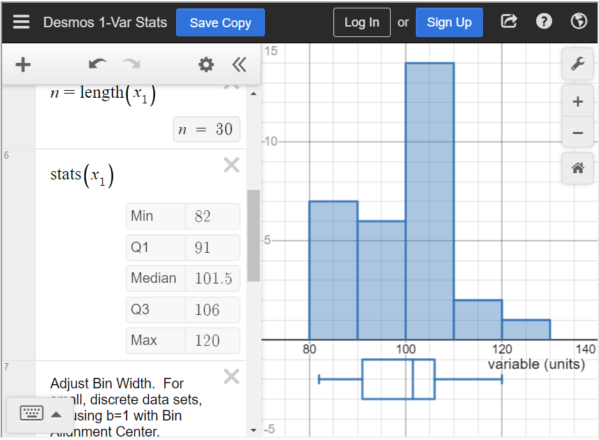
To find the median in the statistics calculator, type all values into [latex]x_1[/latex], separated by a comma. Scroll down until you see “[latex]\text{stats}(x_1)[/latex].” This is the five-number summary of the data. In this table, you can see that the median is 101.5.
Compute the mean of the numbers 12, 15, 17, 18, 18, and 19.
To find the mean in the statistics calculator, type all values into [latex]x_1[/latex], separated by a comma. Below that is a box that says “[latex]x_{bar}=\text{mean}(x_1)[/latex].” This is the mean of the data. You can see that the mean is 16.5.

Refer again to the frequency distribution of the number of siblings people who attended a conflict resolution class reported:
| Number of siblings | Frequency |
|---|---|
| 0 | 5 |
| 1 | 13 |
| 2 | 6 |
| 3 | 3 |
| 4 | 2 |
| 5 | 1 |
What is the mean of the number of siblings?
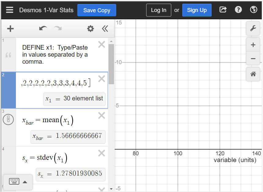
To find the mean in the statistics calculator, type all values into [latex]x_1[/latex], separated by a comma. Because the table is a frequency distribution, we know that 5 people have 0 siblings, 13 people have 1 sibling, and so on. Therefore, be sure to put five 0s, thirteen 1s, and so on. The mean is approximately 1.57.
Examples from Section 8.4
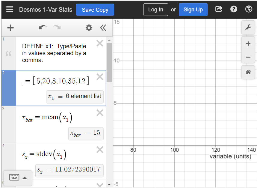
You surveyed some of your friends to find out how many hours they work each week. Their responses were 5, 20, 8, 10, 35, and 12. What is the standard deviation?
To find the standard deviation in the statistics calculator, type all values into [latex]x_1[/latex], separated by a comma. Below that is a box that says “[latex]s_x=\text{stdev}(x_1)[/latex].” This is the standard deviation of the data. You can see that the standard deviation is approximately 11.03.
Media Attributions
- 8.8 01 is licensed under a CC0 (Creative Commons Zero) license
- 8.9 02 is licensed under a CC0 (Creative Commons Zero) license
- 8.8 03 is licensed under a CC0 (Creative Commons Zero) license
- 8.8 04 is licensed under a CC0 (Creative Commons Zero) license
- 8.8 05 is licensed under a CC0 (Creative Commons Zero) license
- 8.8 06 is licensed under a CC0 (Creative Commons Zero) license
- 8.8 07 is licensed under a CC0 (Creative Commons Zero) license
- 8.8 08 is licensed under a CC0 (Creative Commons Zero) license
- 8.8 09 is licensed under a CC0 (Creative Commons Zero) license
