The notation for the chi-square distribution is [latex]\chi \sim {\chi }_{df}^{2}[/latex], where [latex]df = \text{degrees of freedom}[/latex], which depends on how chi-square is being used. (If you want to practice calculating chi-square probabilities then use [latex]df = n - 1[/latex]. The degrees of freedom for the three major uses are each calculated differently.)

For the [latex]\chi^2[/latex] distribution, the population mean is [latex]\mu = df[/latex] and the population standard deviation is [latex]\sigma =\sqrt{2(df)}[/latex].

The random variable is shown as [latex]\chi^2[/latex], but may be any uppercase letter.

The random variable for a chi-square distribution with [latex]k[/latex] degrees of freedom is the sum of [latex]k[/latex] independent, squared standard normal variables.

[latex]\chi^2 = (Z_1)^2+(Z_2)^2+...+(Z_k)^2[/latex]

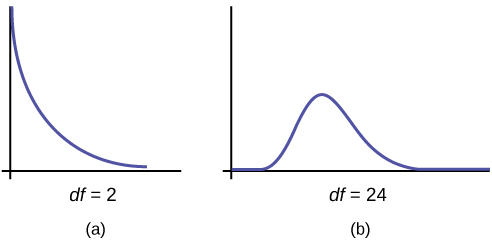
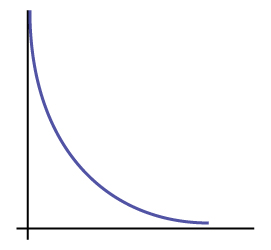
1. The curve is nonsymmetrical and skewed to the right.
2. There is a different chi-square curve for each [latex]df[/latex].
   
3. The test statistic for any test is always greater than or equal to zero.
4. When [latex]df > 90[/latex], the chi-square curve approximates the normal distribution. For [latex]\chi \sim {\chi }_{1,000}^{2}[/latex] the mean, [latex]\mu = df = 1,000[/latex] and the standard deviation, [latex]\sigma = \sqrt{2\left(1,000\right)} = 44.7[/latex]. Therefore, [latex]X \sim N(1,000, 44.7)[/latex], approximately.
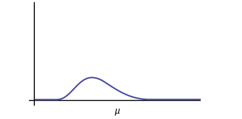
5. The mean, [latex]\mu[/latex], is located just to the right of the peak.
   

Section 11.1 Review

The chi-square distribution is a useful tool for assessment in a series of problem categories. These problem categories include primarily (i) whether a data set fits a particular distribution, (ii) whether the distributions of two populations are the same, (iii) whether two events might be independent, and (iv) whether there is a different variability than expected within a population.

An important parameter in a chi-square distribution is the degrees of freedom [latex]df[/latex] in a given problem. The random variable in the chi-square distribution is the sum of squares of [latex]df[/latex] standard normal variables, which must be independent. The key characteristics of the chi-square distribution also depend directly on the degrees of freedom.

The chi-square distribution curve is skewed to the right, and its shape depends on the degrees of freedom [latex]df[/latex]. For [latex]df > 90[/latex], the curve approximates the normal distribution. Test statistics based on the chi-square distribution are always greater than or equal to zero. Such application tests are almost always right-tailed tests.

Formula Review

Chi-square distribution random variable: [latex]\chi^2 = (Z_1)^2 + (Z_2)^2 + … (Z_{df})^2[/latex]

Chi-square distribution population mean: [latex]\mu_{\chi^2} = df[/latex]

Chi-Square distribution population standard deviation: [latex]{\sigma }_{{\chi }^{2}}\text{=}\sqrt{2\left(df\right)}[/latex]

Section 11.1 Practice

If the number of degrees of freedom for a chi-square distribution is 25, what is the population mean and standard deviation?

Solution

mean = 25 and standard deviation = 7.0711

If [latex]df > 90[/latex], the distribution is [latex]\underline{\hspace{2cm}}[/latex]. If [latex]df = 15[/latex], the distribution is [latex]\underline{\hspace{2cm}}[/latex].

When does the chi-square curve approximate a normal distribution?

Solution

when the number of degrees of freedom is greater than 90

Where is [latex]\mu[/latex] located on a chi-square curve?

Is it more likely the [latex]df[/latex] is 90, 20, or two in the graph?

Solution

[latex]df = 2[/latex]

Decide whether the following statements are true or false.

1. As the number of degrees of freedom increases, the graph of the chi-square distribution looks more and more symmetrical.

Solution

true

 

2. The standard deviation of the chi-square distribution is twice the mean.

 

3. The mean and the median of the chi-square distribution are the same if [latex]df = 24[/latex].

Solution

false

References

Data from Parade Magazine.

“HIV/AIDS Epidemiology Santa Clara County.” Santa Clara County Public Health Department, May 2011.