Chapter 6: The Normal Distribution and The Central Limit Theorem
6.5 The Normal Approximation to the Binomial
Learning Objectives
By the end of this section, the student should be able to:
- Approximate the binomial distribution using the normal distribution
The binomial formula is cumbersome when the sample size ([latex]n[/latex]) is large, particularly when we consider a range of observations. Consider the following example.
Example
Approximately 15% of the US population smokes cigarettes. A local government believed their community had a lower smoker rate and commissioned a survey of 400 randomly selected individuals. The survey found that only 42 of the 400 participants smoke cigarettes. If the true proportion of smokers in the community was really 15%, what is the probability of observing 42 or fewer smokers in a sample of 400 people?
Solution
We first need to verify the four conditions for the binomial model are met. The question posed is equivalent to asking, what is the probability of observing [latex]k = 0, 1, 2, ..., or 42[/latex] smokers in a sample of [latex]n = 400[/latex] when [latex]p = 0.15[/latex]? We can compute these 43 different probabilities and add them together.
[latex]P(k = 0 \text{ or } k = 1 \text{ or } ... \text{ or } k = 42)[/latex]
[latex]= P(k = 0) + P(k = 1) + ... + P(k = 42)[/latex]
[latex]= 0.0054[/latex]
The computations in the previous example are tedious, long, and near impossible if you do not have access to technology. Luckily, we have discovered the [latex]\text{binomcdf()}[/latex] function previously, so this problem with the technology is not horrible to do (Try it for yourself: [latex]\text{binomcdf}(400, 0.15, 42) = 0.0054[/latex]).
In some cases we may use the normal distribution as an easier and faster way to estimate binomial probabilities. In general, we should avoid such work if an alternative method exists that is faster, easier, and still accurate. Recall that calculating probabilities of a range of values is much easier in the normal model. We might wonder, is it reasonable to use the normal model in place of the binomial distribution? Surprisingly, yes, if certain conditions are met.
Historical Note
Historically, being able to compute binomial probabilities was one of the most important applications of the central limit theorem. Binomial probabilities with a small value for [latex]n[/latex] (say, 20) were displayed in a table in a book. To calculate the probabilities with large values of [latex]n[/latex], you had to use the binomial formula, which could be very complicated. Using the normal approximation to the binomial distribution simplified the process.
To compute the normal approximation to the binomial distribution, take a simple random sample from a population. You must meet the conditions for a binomial distribution:
- there are a certain number [latex]n[/latex] of independent trials
- the outcomes of any trial are success or failure
- each trial has the same probability of a success [latex]p[/latex]
Recall that if [latex]X[/latex] is the binomial random variable, then [latex]X \sim B(n, p)[/latex]. The shape of the binomial distribution needs to be similar to the shape of the normal distribution. To ensure this, the quantities [latex]np[/latex] and [latex]nq[/latex] must both be greater than five ([latex]np > 5[/latex] and [latex]nq > 5[/latex]; the approximation is better if they are both greater than or equal to 10). Then the binomial can be approximated by the normal distribution with mean [latex]\mu = np[/latex] and standard deviation [latex]\sigma = \sqrt{npq}[/latex]. Remember that [latex]q = 1 – p[/latex].
Binomial Approximation Conditions
Consider the binomial model when the probability of a success is [latex]p = 0.10[/latex]. The following figures show four hollow histograms for simulated samples from the binomial distribution using four different sample sizes: [latex]n = 10, 30, 100, 300[/latex]. What happens to the shape of the distributions as the sample size increases? What distribution does the last histogram resemble?
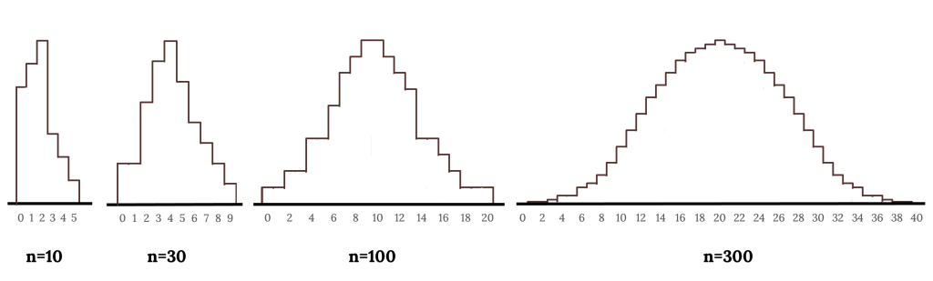
It appears the distribution is transformed from a blocky and skewed distribution into one that rather resembles the normal distribution in the last hollow histogram.
The binomial distribution with probability of success p is nearly normal when the sample size n is sufficiently large that [latex]np[/latex] and [latex]n(1 − p)[/latex] are both at least 10. The approximate normal distribution has parameters corresponding to the mean and standard deviation of the binomial distribution: [latex]\mu = np[/latex] and [latex]\sigma = \sqrt{np(1 − p)}[/latex]
The normal approximation may be used when computing the range of many possible successes. For instance, we may apply the normal distribution to the setting of the previous example:
Example
Use the normal approximation to estimate the probability of observing 42 or fewer smokers in a sample of 400, if the true proportion of smokers is [latex]p = 0.15[/latex].
Already knowing that the binomial model, we then verify that both [latex]np[/latex] and [latex]n(1 − p)[/latex] are at least 10:
- [latex]np = 400 \times 0.15 = 60 n(1 − p) = 400 \times 0.85 = 340[/latex]
With these conditions met, we may use the normal approximation in place of the binomial distribution using the mean and standard deviation from the binomial model:
- [latex]\mu = np = 60[/latex] and [latex]\sigma =\sqrt{np(1 − p)} = \sqrt{60(1-.015)} = 7.14[/latex]
We want to find the probability of observing 42 or fewer smokers using this model. Use the normal model [latex]N(\mu = 60, \sigma = 7.14)[/latex] and standardize to estimate the probability of observing 42 or fewer smokers. Your answer should be approximately equal to the solution we found in the previous example, 0.0054.
Compute the Z-score first:
Solution
[latex]Z =\frac{(42−60)}{7.14} = -2.52[/latex]
The corresponding left tail area from the table or technology is 0.0059.
The Continuity Correction
The normal approximation to the binomial distribution tends to perform poorly when estimating the probability of a small range of counts, even when the conditions are met.
Suppose we wanted to compute the probability of observing 49, 50, or 51 smokers in 400 when [latex]p = 0.15[/latex]. With such a large sample, we might be tempted to apply the normal approximation and use the range 49 to 51. However, we would find that the binomial solution and the normal approximation notably differ:
- Binomial: 0.0649
- Normal: 0.0421
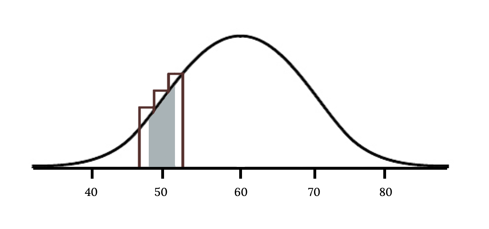
We can identify the cause of this discrepancy in the next figure which shows the areas representing the binomial probability (outlined) and normal approximation (shaded). Notice that the width of the area under the normal distribution is 0.5 units too slim on both sides of the interval.

The normal approximation to the binomial distribution for intervals of values can usually be improved if cutoff values are modified slightly. The cutoff values for the lower end of a shaded region should be reduced by 0.5, and the cutoff value for the upper end should be increased by 0.5. This is called the continuity correction.
The tip to add extra area when applying the normal approximation is most often useful when examining a range of observations. In the example above, the revised normal distribution estimate is 0.0633, much closer to the exact value of 0.0649. While it is possible to also apply this correction when computing a tail area, the benefit of the modification usually disappears since the total interval is typically quite wide. So, in order to get the best approximation, add 0.5 to x or subtract 0.5 from x (use [latex]x + 0.5[/latex] or [latex]x – 0.5[/latex]). The number 0.5 is called the continuity correction factor and is used in the following example.
Example
Suppose in a local Kindergarten through 12th grade (K – 12) school district, 53 percent of the population favor a charter school for grades K through 5. A simple random sample of 300 is surveyed.
- Find the probability that at least 150 favor a charter school.
- Find the probability that at most 160 favor a charter school.
- Find the probability that more than 155 favor a charter school.
- Find the probability that fewer than 147 favor a charter school.
- Find the probability that exactly 175 favor a charter school.
Let [latex]X =[/latex] the number that favors a charter school for grades K through 5. [latex]X \sim B(n, p)[/latex] where [latex]n = 300[/latex] and [latex]p = 0.53[/latex]. Since [latex]np > 5[/latex] and [latex]nq > 5[/latex], use the normal approximation to the binomial.
Remember, the formulas for the mean and standard deviation are [latex]\mu = np[/latex] and [latex]\sigma =\sqrt{npq}[/latex]. The mean is 159 and the standard deviation is 8.6447. The random variable for the normal distribution is [latex]Y: Y \sim N(159, 8.6447)[/latex].
Remember in Section 6.2, we learned how to use the [latex]\text{normalcdf()}[/latex] function in the graphing calculator:
Using the TI-83+ and TI-84 Calculators for Normal Probabilities
Go into 2nd DISTR.
Press 2: normalcdf.
The syntax for the instructions are as follows: [latex]\text{normalcdf(lower value, upper value, mean, standard deviation)}[/latex]
In some instances:
- the upper number of the area might be [latex]1\text{E}99[/latex] (which equals [latex]10^{99}[/latex]). You get [latex]1\text{E}99 = 10^{99})[/latex] by pressing [latex]1[/latex], the [latex]\text{EE}[/latex] key (a 2nd key) and then [latex]99[/latex]. Or, you can enter [latex]10^{99}[/latex] instead. The number [latex]10^{99}[/latex] is way out in the right tail of the normal curve.
- the lower number of the area might be [latex]-1 \text{E} 99[/latex] (which equals [latex]-10^{99}[/latex]). The number [latex]-10^{99}[/latex] is way out in the left tail of the normal curve.
Use that function for this problem!
Solution
- Include 150 so [latex]P(X \ge 150)[/latex] has normal approximation [latex]P(Y \ge 149.5) = 0.8641[/latex]
[latex]\text{normalcdf}(149.5, 10^{99}, 159, 8.6447) = 0.8641[/latex]. - Include 160 so [latex]P(X \le 160)[/latex] has normal approximation [latex]P(Y \le 160.5) = 0.5689[/latex].
[latex]\text{normalcdf}(0, 160.5, 159, 8.6447) = 0.5689[/latex] - Exclude 155 so [latex]P(X > 155)[/latex] has normal approximation [latex]P(Y > 155.5) = 0.6572[/latex].[latex]\text{normalcdf}(155.5, 10^{99}, 159, 8.6447) = 0.6572[/latex]
- Exclude 147 so [latex]P(X \lt 147)[/latex] has normal approximation [latex]P(Y \lt 146.5) = 0.0741[/latex].
[latex]\text{normalcdf}(0, 146.5, 159, 8.6447) = 0.0741[/latex] - [latex]P(X = 175)[/latex] has normal approximation [latex]P(174.5 \lt Y \lt 175.5) = 0.0083[/latex].
[latex]\text{normalcdf}(174.5, 175.5, 159, 8.6447) = 0.0083[/latex]
Note
Because of calculators and computer software that let you calculate binomial probabilities for large values of n easily, it is not necessary to use the normal approximation to the binomial distribution, provided that you have access to these technology tools. Most school labs have Microsoft Excel, an example of computer software that calculates binomial probabilities. Many students have access to the TI-83 or 84 series calculators, and they easily calculate probabilities for the binomial distribution. If you type in “binomial probability distribution calculation” in an Internet browser, you can find at least one online calculator for the binomial.
For the previous example, the probabilities are calculated using the following binomial distribution: ([latex]n = 300[/latex] and [latex]p = 0.53[/latex]). Compare the binomial and normal distribution answers.
[latex]P(X \ge 150) : 1 - \text{binomcdf}(300, 0.53, 149) = 0.8641[/latex]
[latex]P(X \le 160) : \text{binomcdf}(300, 0.53, 160) = 0.5684[/latex]
[latex]P(X > 155) : 1 - \text{binomcdf}(300, 0.53, 155) = 0.6576[/latex]
[latex]P(X \lt 147) : \text{binomcdf}(300, 0.53, 146) = 0.0742[/latex]
[latex]P(X = 175) : \text{binomcdf}(300, 0.53, 175) = 0.0083[/latex]
Your Turn!
In a city, 46 percent of the population favor the incumbent, Dawn Morgan, for mayor. A simple random sample of 500 is taken. Using the continuity correction factor, find the probability that at least 250 favor Dawn Morgan for mayor.
Solution
0.0401
Section 6.5 Review
The central limit theorem can be used to illustrate the law of large numbers. The law of large numbers states that the larger the sample size you take from a population, the closer the sample mean [latex]\overline{x}[/latex] gets to [latex]\mu[/latex].
Section 6.5 Practice
Use the following information to answer the next ten exercises:
A manufacturer produces 25-pound lifting weights. The lowest actual weight is 24 pounds, and the highest is 26 pounds. Each weight is equally likely so the distribution of weights is uniform. A sample of 100 weights is taken.
1. Answer the following:
a. What is the distribution for the weights of one 25-pound lifting weight? What is the mean and standard deviation?
b. What is the distribution for the mean weight of 100 25-pound lifting weights?
c. Find the probability that the mean actual weight for the 100 weights is less than 24.9.
Solution
a. [latex]U(24, 26), 25, 0.5774[/latex]
b. [latex]N(25, 0.0577)[/latex]
c. 0.0416
2. Find the probability that the mean actual weight for the 100 weights is greater than 25.2.
Solution
0.0003
3. Find the 90th percentile for the mean weight for the 100 weights.
Solution
25.07
4. Answer the following:
a. What is the distribution for the sum of the weights of 100 25-pound lifting weights?
b. Find [latex]P(\Sigma{X} \lt 2,450)[/latex].
Solution
a. [latex]N(2,500, 5.7735)[/latex]
b. 0
5. Find the 90th percentile for the total weight of the 100 weights.
Solution
2,507.40
Use the following information to answer the next eight exercises:
The length of time a particular smartphone’s battery lasts follows an exponential distribution with a mean of ten months. A sample of 64 of these smartphones is taken.
1. Answer the following:
a. What is the standard deviation?
b. What is the parameter [latex]m[/latex]?
Solution
a. 10
b. [latex]\frac{1}{10}[/latex]
2. What is the distribution for the length of time one battery lasts?
Solution
Exp(1/10)
3. What is the distribution for the mean length of time 64 batteries last?
Solution
[latex]N \left(10, \frac{10}{8}\right)[/latex]
4. What is the distribution for the total length of time 64 batteries last?
Solution
[latex]N(640, 80)[/latex]
5. Find the probability that the sample mean is between seven and 11.
Solution
0.7799
6. Find the 80th percentile for the total length of time 64 batteries last.
Solution
707.3
7. Find the IQR for the mean amount of time 64 batteries last.
Solution
1.69
8. Find the middle 80% for the total amount of time 64 batteries last.
Solution
between 537.48 and 742.52
Use the following information to answer the next six exercises:
A uniform distribution has a minimum of six and a maximum of ten. A sample of 50 is taken.
1. Find [latex]P(\Sigma{X} > 420)[/latex].
Solution
0.0072
2. Find the 90th percentile for the sums.
Solution
410.46
3. Find the 15th percentile for the sums.
Solution
391.54
4. Find the first quartile for the sums.
Solution
394.49
5. Find the third quartile for the sums.
Solution
405.51
Find the 80th percentile for the sums.
Solution
406.87
The attention span of a two-year-old is exponentially distributed with a mean of about eight minutes. Suppose we randomly survey 60 two-year-olds.
- In words, [latex]X = \underline{\hspace{2cm}}[/latex]
- [latex]X \sim \underline{\hspace{2cm}}(\underline{\hspace{2cm}}, \underline{\hspace{2cm}})[/latex]
- In words, [latex]\overline{X} = \underline{\hspace{2cm}}[/latex]
- [latex]\overline{X} \sim \underline{\hspace{2cm}}(\underline{\hspace{2cm}}, \underline{\hspace{2cm}})[/latex]
- Before doing any calculations, which do you think will be higher? Explain why.
- The probability that an individual attention span is less than ten minutes.
- The probability that the average attention span for the 60 children is less than ten minutes?
- Calculate the probabilities in part e.
- Explain why the distribution for [latex]\overline{X}[/latex] is not exponential.
Solution
- [latex]X =[/latex] the attention span of a two-year-old
- [latex]Χ \sim Exp(18)[/latex]
- [latex]\overline{X}= \text{the mean (average) attention span of a two-year-old}[/latex]
- [latex]\overline{X} \sim N(8, 860)[/latex]
- The standard deviation is smaller, so there is more area under the normal curve.
- Exponential: 0.7135
- Normal: 0.7579
- By the central limit theorem, as n gets larger, the means tend to follow a normal distribution.
The closing stock prices of 35 U.S. semiconductor manufacturers are given as follows.
8.625; 30.25; 27.625; 46.75; 32.875; 18.25; 5; 0.125; 2.9375; 6.875; 28.25; 24.25; 21; 1.5; 30.25; 71; 43.5; 49.25; 2.5625; 31; 16.5; 9.5; 18.5; 18; 9; 10.5; 16.625; 1.25; 18; 12.87; 7; 12.875; 2.875; 60.25; 29.25
- In words, [latex]Χ = \underline{\hspace{2cm}}[/latex]
- [latex]\overline{x} = \underline{\hspace{2cm}}[/latex]
- [latex]s_x = \underline{\hspace{2cm}}[/latex]
- [latex]n = \underline{\hspace{2cm}}[/latex]
- Construct a histogram of the distribution of the averages. Start at [latex]x = -0.0005[/latex]. Use bar widths of ten.
- In words, describe the distribution of stock prices.
- Randomly average five stock prices together. (Use a random number generator.) Continue averaging five pieces together until you have ten averages. List those ten averages.
- Use the ten averages from part e to calculate the following.
- [latex]\overline{x} = \underline{\hspace{2cm}}[/latex]
- [latex]s_x = \underline{\hspace{2cm}}[/latex]
- Construct a histogram of the distribution of the averages. Start at [latex]x = -0.0005[/latex]. Use bar widths of ten.
- Does this histogram look like the graph in part c?
- In one or two complete sentences, explain why the graphs either look the same or look different?
- Based upon the theory of the central limit theorem, [latex]\overline{X} \sim \underline{\hspace{2cm}}(\underline{\hspace{2cm}}, \underline{\hspace{2cm}})[/latex]
Solution
- [latex]X =[/latex] the closing stock prices for U.S. semiconductor manufacturers
- $20.71
- $17.31
- $35
- Check student solutions
- Exponential distribution, [latex]X \sim \text{Exp}\left(\frac{1}{20.71}\right)[/latex]
- Answers will vary.
- i. $20.71; ii. $11.14
- Answers will vary.
- Answers will vary.
- Answers will vary.
- [latex]N \left(20.71, \frac{17.31}{\sqrt{5}}\right)[/latex]
Use the following information to answer the next three exercises:
Richard’s Furniture Company delivers furniture from 10 A.M. to 2 P.M. continuously and uniformly. We are interested in how long (in hours) past the 10 A.M. start time that individuals wait for their delivery.
1. [latex]X \sim \underline{\hspace{2cm}}(\underline{\hspace{2cm}}, \underline{\hspace{2cm}})[/latex]
a. [latex]U(0,4)[/latex]
b. [latex]U(10,2)[/latex]
c. [latex]\text{Exp}(2)[/latex]
d. [latex]N(2,1)[/latex]
Solution
a. [latex]U(0,4)[/latex]
2. The average wait time is:
a. one hour.
b. two hours.
c. two and a half hours.
d. four hours.
Solution
b. two hours
3. Suppose that it is now past noon on a delivery day. The probability that a person must wait at least one and a half more hours is:
a. [latex]\frac{1}{4}[/latex]
b. [latex]\frac{1}{2}[/latex]
c. [latex]\frac{3}{4}[/latex]
d. [latex]\frac{3}{8}[/latex]
Solution
a. [latex]\frac{1}{4}[/latex]
Use the following information to answer the next two exercises:
The time to wait for a particular rural bus is distributed uniformly from zero to 75 minutes. One hundred riders are randomly sampled to learn how long they waited.
1. The 90th percentile sample average wait time (in minutes) for a sample of 100 riders is:
a. 315.0
b. 40.3
c. 38.5
d. 65.2
Solution
40.3b.
2. Would you be surprised, based upon numerical calculations, if the sample average wait time (in minutes) for 100 riders was less than 30 minutes?
a. yes
b. no
c. There is not enough information.
Solution
a. yes
Use the following to answer the next two exercises:
The cost of unleaded gasoline in the Bay Area once followed an unknown distribution with a mean of $4.59 and a standard deviation of $0.10. Sixteen gas stations from the Bay Area are randomly chosen. We are interested in the average cost of gasoline for the 16 gas stations.
What’s the approximate probability that the average price for 16 gas stations is over $4.69?
a. almost zero
b. 0.1587
c. 0.0943
d. unknown
Solution
a. almost zero
Find the probability that the average price for 30 gas stations is less than $4.55.
a. 0.6554
b. 0.3446
c. 0.0142
d. 0.9858
e. 0
Solution
c. 0.0142
Suppose in a local Kindergarten through 12th grade (K – 12) school district, 53 percent of the population favor a charter school for grades K through five. A simple random sample of 300 is surveyed. Calculate following using the normal approximation to the binomial distribution.
- Find the probability that less than 100 favor a charter school for grades K through 5.
- Find the probability that 170 or more favor a charter school for grades K through 5.
- Find the probability that no more than 140 favor a charter school for grades K through 5.
- Find the probability that there are fewer than 130 that favor a charter school for grades K through 5.
- Find the probability that exactly 150 favor a charter school for grades K through 5.
If you have access to an appropriate calculator or computer software, try calculating these probabilities using the technology.
Solution
- 0
- 0.1123
- 0.0162
- 0.0003
- 0.0268
Four friends, Janice, Barbara, Kathy and Roberta, decided to carpool together to get to school. Each day the driver would be chosen by randomly selecting one of the four names. They carpool to school for 96 days. Use the normal approximation to the binomial to calculate the following probabilities. Round the standard deviation to four decimal places.
- Find the probability that Janice is the driver for at most 20 days.
- Find the probability that Roberta is the driver for more than 16 days.
- Find the probability that Barbara drives exactly 24 of those 96 days.
Solution
- 0.2047
- 0.9615
- 0.0938
[latex]X \sim N(60, 9)[/latex]. Suppose that you form random samples of 25 from this distribution. Let [latex]\overline{X}[/latex] be the random variable of averages. Let ΣX be the random variable of sums. For parts c through f, sketch the graph, shade the region, label and scale the horizontal axis for [latex]\overline{X}[/latex], and find the probability.
- Sketch the distributions of X and [latex]\overline{X}[/latex] on the same graph.
- [latex]\overline{X} \sim \underline{\hspace{2cm}}(\underline{\hspace{2cm}}, \underline{\hspace{2cm}})[/latex]
- [latex]P(\overline{x} \lt 60) = \underline{\hspace{2cm}}[/latex]
- Find the 30th percentile for the mean.
- [latex]P(56 \lt \overline{x} \lt 62) = \underline{\hspace{2cm}}[/latex]
- [latex]P(18 \lt \overline{x} \lt 58) = \underline{\hspace{2cm}}[/latex]
- [latex]\Sigma{x} \sim \underline{\hspace{2cm}}(\underline{\hspace{2cm}},\underline{\hspace{2cm}})[/latex]
- Find the minimum value for the upper quartile for the sum.
- [latex]P(1,400 \lt \Sigma{x} \lt 1,550) = \underline{\hspace{2cm}}[/latex]
Solution
- Check student’s solution.
- [latex]\overline{X} \sim N \left(60, \frac{9}{\sqrt{25}}\right)[/latex]
- 0.5000
- 59.06
- 0.8536
- 0.1333
- [latex]N(1500, 45)[/latex]
- 1530.35
- 0.6877
Salaries for teachers in a particular elementary school district are normally distributed with a mean of $44,000 and a standard deviation of $6,500. We randomly survey ten teachers from that district.
- Find the 90th percentile for an individual teacher’s salary.
- Find the 90th percentile for the average teacher’s salary.
Solution
- $52,330
- $46,634
The average length of a maternity stay in a U.S. hospital is said to be 2.4 days with a standard deviation of 0.9 days. We randomly survey 80 women who recently bore children in a U.S. hospital.
- In words, [latex]X = \underline{\hspace{2cm}}[/latex]
- In words, [latex]\overline{X} = \underline{\hspace{2cm}}[/latex]
- [latex]\overline{X} \sim \underline{\hspace{2cm}}(\underline{\hspace{2cm}}, \underline{\hspace{2cm}})[/latex]
- In words, [latex]\Sigma{X} = \underline{\hspace{2cm}}[/latex]
- [latex]\Sigma{X} \sim \underline{\hspace{2cm}}(\underline{\hspace{2cm}}, \underline{\hspace{2cm}})[/latex]
- Is it likely that an individual stayed more than five days in the hospital? Why or why not?
- Is it likely that the average stay for the 80 women was more than five days? Why or why not?
- Which is more likely:
a. An individual stayed more than five days.
b. The average stay of 80 women was more than five days. - If we were to sum up the women’s stays, is it likely that, collectively, they spent more than a year in the hospital? Why or why not?
Solution
- the length of a maternity stay in a U.S. hospital, in days
- the average length of a maternity stay in a U.S. hospital, in days
- [latex]N(2.4, 0.980)[/latex]
- the total of the 80 women’s length of maternity stay in a U.S. hospital, in days
- [latex]N(192, 8.05)[/latex]
- Not likely, but possible. The mean stay is 2.4 days.
- No, the probability is 0.
- a. An individual stayed more than five days.
- No, the probability is 0.
For each problem, wherever possible, provide graphs and use the calculator.
1. NeverReady batteries has engineered a newer, longer lasting AAA battery. The company claims this battery has an average life span of 17 hours with a standard deviation of 0.8 hours. Your statistics class questions this claim. As a class, you randomly select 30 batteries and find that the sample mean life span is 16.7 hours. If the process is working properly, what is the probability of getting a random sample of 30 batteries in which the sample mean lifetime is 16.7 hours or less? Is the company’s claim reasonable?
Solution
- We have [latex]\mu = 17[/latex], [latex]\sigma = 0.8[/latex], [latex]\overline{x}= 16.7[/latex], and [latex]n = 30[/latex]. To calculate the probability, we use \text{normalcdf(lower, upper, }\mu, [latex]\frac{\sigma }{\sqrt{n}}) = \text{normalcdf}\left(\text{E}-99, 16.7,17,\frac{0.8}{\sqrt{30}}\right) = 0.0200[/latex].
- If the process is working properly, then the probability that a sample of 30 batteries would have at most 16.7 lifetime hours is only 2%. Therefore, the class was justified to question the claim.
2. Men have an average weight of 172 pounds with a standard deviation of 29 pounds.
- Find the probability that 20 randomly selected men will have a sum weight greater than 3,600 lbs.
- If 20 men have a sum weight greater than 3,500 lbs., then their total weight exceeds the safety limits for water taxis. Based on (a), is this a safety concern? Explain.
Solution
To calculate the probability, we use [latex]\text{normalcdf}(3600, \text{E}99, 3440, 129.69) = 0.1087[/latex]
While the probability is not exceptionally large, [latex]P(\overline{X} > 3600) = 0.1087[/latex], it could be wise to be concerned. After all, we do have a 1 in 10 chance that a random sample of men could have an average sum weight that exceeds the safety limit.
3. M&M candies large candy bags have a claimed net weight of 396.9 g. The standard deviation for the weight of the individual candies is 0.017 g. The following table is from a stats experiment conducted by a statistics class.
| Red | Orange | Yellow | Brown | Blue | Green |
|---|---|---|---|---|---|
| 0.751 | 0.735 | 0.883 | 0.696 | 0.881 | 0.925 |
| 0.841 | 0.895 | 0.769 | 0.876 | 0.863 | 0.914 |
| 0.856 | 0.865 | 0.859 | 0.855 | 0.775 | 0.881 |
| 0.799 | 0.864 | 0.784 | 0.806 | 0.854 | 0.865 |
| 0.966 | 0.852 | 0.824 | 0.840 | 0.810 | 0.865 |
| 0.859 | 0.866 | 0.858 | 0.868 | 0.858 | 1.015 |
| 0.857 | 0.859 | 0.848 | 0.859 | 0.818 | 0.876 |
| 0.942 | 0.838 | 0.851 | 0.982 | 0.868 | 0.809 |
| 0.873 | 0.863 | 0.803 | 0.865 | ||
| 0.809 | 0.888 | 0.932 | 0.848 | ||
| 0.890 | 0.925 | 0.842 | 0.940 | ||
| 0.878 | 0.793 | 0.832 | 0.833 | ||
| 0.905 | 0.977 | 0.807 | 0.845 | ||
| 0.850 | 0.841 | 0.852 | |||
| 0.830 | 0.932 | 0.778 | |||
| 0.856 | 0.833 | 0.814 | |||
| 0.842 | 0.881 | 0.791 | |||
| 0.778 | 0.818 | 0.810 | |||
| 0.786 | 0.864 | 0.881 | |||
| 0.853 | 0.825 | ||||
| 0.864 | 0.855 | ||||
| 0.873 | 0.942 | ||||
| 0.880 | 0.825 | ||||
| 0.882 | 0.869 | ||||
| 0.931 | 0.912 | ||||
| 0.887 |
The bag contained 465 candies, and the listed weights in the table came from randomly selected candies. Count the weights.
- Find the mean sample weight and the standard deviation of the sample weights of candies in the table.
- Find the sum of the sample weights in the table and the standard deviation of the sum of the weights.
- If 465 M&Ms are randomly selected, find the probability that their weights sum to at least 396.9.
- Is the Mars Company’s M&M labeling accurate?
Solution
- For the sample, we have [latex]n = 100[/latex], [latex]\overline{x} = 0.862[/latex], [latex]s = 0.05[/latex]
- [latex]\Sigma \overline{x} = 85.65[/latex], [latex]\Sigma{s} = 5.18[/latex]
- [latex]\text{normalcdf}(396.9, \text{E}99, (465)(0.8565), (0.05)(\sqrt{465})) \approx 1[/latex]
- Since the probability of a sample of size 465 having at least a mean sum of 396.9 is approximately 1, we can conclude that Mars is correctly labeling their M&M packages.
4. The Screw Right Company claims their [latex]\frac{3}{4}[/latex]-inch screws are within ±0.23 of the claimed mean diameter of 0.750 inches with a standard deviation of 0.115 inches. The following data were recorded.
| 0.757 | 0.723 | 0.754 | 0.737 | 0.757 | 0.741 | 0.722 | 0.741 | 0.743 | 0.742 |
| 0.740 | 0.758 | 0.724 | 0.739 | 0.736 | 0.735 | 0.760 | 0.750 | 0.759 | 0.754 |
| 0.744 | 0.758 | 0.765 | 0.756 | 0.738 | 0.742 | 0.758 | 0.757 | 0.724 | 0.757 |
| 0.744 | 0.738 | 0.763 | 0.756 | 0.760 | 0.768 | 0.761 | 0.742 | 0.734 | 0.754 |
| 0.758 | 0.735 | 0.740 | 0.743 | 0.737 | 0.737 | 0.725 | 0.761 | 0.758 | 0.756 |
The screws were randomly selected from the local home repair store.
- Find the mean diameter and standard deviation for the sample
- Find the probability that 50 randomly selected screws will be within the stated tolerance levels. Is the company’s diameter claim plausible?
Solution
[latex]\overline{x}= 0.75[/latex] and [latex]s = 0.01[/latex]
We have [latex]\text{normalcdf}(0.52, 0.98, 0.75, 0.11550) \approx 1[/latex] and we can conclude that the company’s diameter claim is justified.
5. Your company has a contract to perform preventive maintenance on thousands of air-conditioners in a large city. Based on service records from previous years, the time that a technician spends servicing a unit averages one hour with a standard deviation of one hour. In the coming week, your company will service a simple random sample of 70 units in the city. You plan to budget an average of 1.1 hours per technician to complete the work. Will this be enough time?
Solution
Use [latex]\text{normalcdf} \left(\text{E} - 99, 1.1, 1, \frac{1}{\sqrt{70}} \right) = 0.7986[/latex]. This means that there is an 80% chance that the service time will be less than 1.1 hours. It could be wise to schedule more time since there is an associated 20% chance that the maintenance time will be greater than 1.1 hours.
6. A typical adult has an average IQ score of 105 with a standard deviation of 20. If 20 randomly selected adults are given an IQ test, what is the probability that the sample mean scores will be between 85 and 125 points?
Solution
The probability that the sample score is between 85 and 125 points is given by [latex]\text{normalcdf}(85, 125, 105, 2020)= 0.9999[/latex]. Therefore, it is almost a guarantee that a well selected sample of 20 adults will have an average score between 85 and 125.
7. Certain coins have an average weight of 5.201 grams with a standard deviation of 0.065 g. If a vending machine is designed to accept coins whose weights range from 5.111 g to 5.291 g, what is the expected number of rejected coins when 280 randomly selected coins are inserted into the machine?
Solution
Since we have [latex]\text{normalcdf} \left(5.111, 5.291, 5.201, \frac{0.\text{065}}{\sqrt{280}} \right) \approx 1[/latex], we can conclude that practically all the coins are within the limits, therefore, there should be no rejected coins out of a well selected sample of size 280.
References
Data from the Wall Street Journal.
“National Health and Nutrition Examination Survey.” Center for Disease Control and Prevention. Available online at http://www.cdc.gov/nchs/nhanes.htm (accessed May 17, 2013).
Media Attributions
- Private: Figure 5.14 © Significant Statistics by John Morgan Russell is licensed under a CC BY-SA (Attribution ShareAlike) license
- Private: Figure 5.15 © Significant Statistics by John Morgan Russell is licensed under a CC BY-SA (Attribution ShareAlike) license
A random variable that counts the number of successes in a fixed number (n) of independent Bernoulli trials each with probability of a success (p)
When statisticians add or subtract .5 to values to improve approximation
