Chapter 6: The Normal Distribution and The Central Limit Theorem
6.1 The Standard Normal Distribution
Learning Objectives
By the end of this section, the student should be able to:
- Calculate and interpret z-scores.
- Recognize characteristics of the standard normal distribution.
- Apply the empirical rule to solve real-world applications.
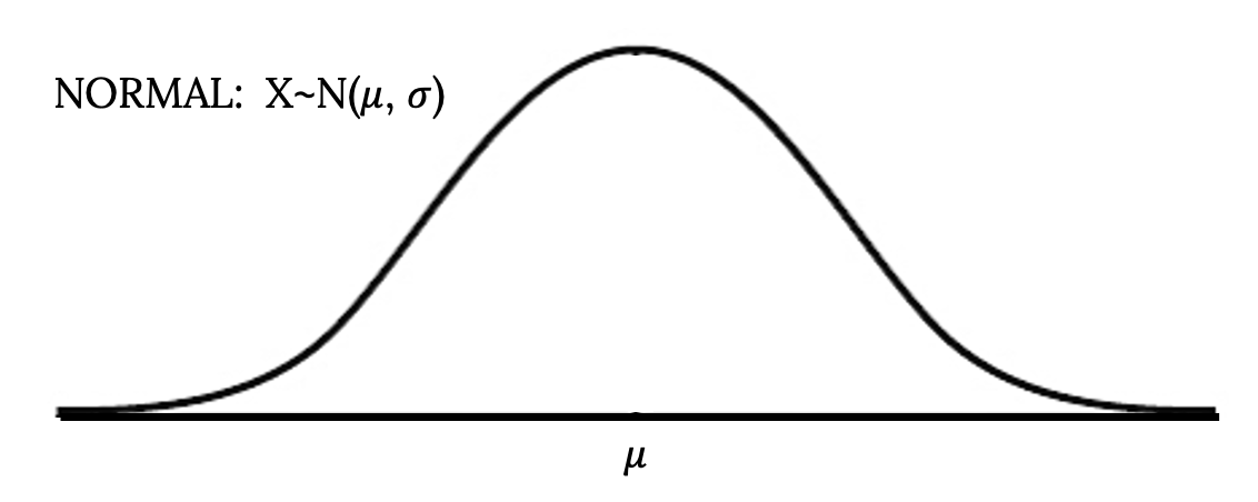
The normal distribution has two parameters (two numerical descriptive measures): the mean (μ) and the standard deviation (σ). If X is a quantity to be measured that has a normal distribution with mean (μ) and standard deviation (σ), we designate this by writing X~N(μ, σ).

The probability density function of this curve is as follows:
f(x) = [latex]\frac{1}{\sigma \cdot \sqrt{2\cdot \pi }} \cdot {\text{ e}}^{-\frac{1}{2}\cdot {\left(\frac{x-\mu }{\sigma }\right)}^{2}}[/latex]
where:
- -∞ < X < ∞
- -∞ < μ < ∞
- σ > 0
As you can see, the normal pdf is a rather complicated function. Do not memorize it. It is not necessary. But this could be a problem since the normal distribution is so widely used. However we will see some ways we can work around this.
The cumulative distribution function is P(X < x). It is calculated either by a calculator or a computer, or it is looked up in a table. Technology has made the tables virtually obsolete.
The curve is symmetrical about a vertical line drawn through the mean, μ. In theory, the mean is the same as the median, because the graph is symmetric about μ. As the notation indicates, the normal distribution depends only on the mean and the standard deviation. Since the area under the curve must equal one, a change in the standard deviation, σ, causes a change in the shape of the curve; the curve becomes fatter or skinnier depending on σ. A change in μ causes the graph to shift to the left or right. This means there are an infinite number of normal probability distributions. One of special interest is called the standard normal distribution.
The standard normal distribution is a normal distribution of standardized values called z-scores. A z-score is measured in units of the standard deviation. For example, if the mean of a normal distribution is five and the standard deviation is two, the value 11 is three standard deviations above (or to the right of) the mean. The calculation is as follows:
x = μ + (z)(σ) = 5 + (3)(2) = 11
The z-score is three.
The mean for the standard normal distribution is zero, and the standard deviation is one. The transformation z = [latex]\frac{x-\mu }{\sigma }[/latex] produces the distribution Z ~ N(0, 1). The value x comes from a normal distribution with mean μ and standard deviation σ.
Z-Scores
If X is a normally distributed random variable and X ~ N(μ, σ), then the z-score is:
The z-score tells you how many standard deviations the value x is above (to the right of) or below (to the left of) the mean, μ. Values of x that are larger than the mean have positive z-scores, and values of x that are smaller than the mean have negative z-scores. If x equals the mean, then x has a z-score of zero.
Note
Suppose X ~ N(5, 6). This says that x is a normally distributed random variable with mean μ = 5 and standard deviation σ = 6. Suppose x = 17.
Then: [latex]z=\frac{x–\mu }{\sigma }=\frac{17–5}{6}=2[/latex]
This means that x = 17 is two standard deviations (2σ) above or to the right of the mean μ = 5. The standard deviation is σ = 6.
Notice that: 5 + (2)(6) = 17 (The pattern is μ + zσ = x)
Now suppose x = 1. Then: z = [latex]\frac{x–\mu }{\sigma }[/latex] = [latex]\frac{1–5}{6}[/latex] = –0.67 (rounded to two decimal places)
This means that x = 1 is 0.67 standard deviations (–0.67σ) below or to the left of the mean μ = 5. Notice that: 5 + (–0.67)(6) is approximately equal to one (This has the pattern μ + (–0.67)σ = 1)
Summarizing, when z is positive, x is above or to the right of μ and when z is negative, x is to the left of or below μ. Or, when z is positive, x is greater than μ, and when z is negative x is less than μ.
Example
Some doctors believe that a person can lose five pounds, on the average, in a month by reducing his or her fat intake and by exercising consistently. Suppose weight loss has a normal distribution. Let X = the amount of weight lost(in pounds) by a person in a month. Use a standard deviation of two pounds. X ~ N(5, 2). Fill in the blanks.
a. Suppose a person lost ten pounds in a month. The z-score when x = 10 pounds is z = 2.5 (verify). This z-score tells you that x = 10 is ________ standard deviations to the ________ (right or left) of the mean _____ (What is the mean?).
Solution
This z-score tells you that x = 10 is 2.5 standard deviations to the right of the mean five.
b. Suppose a person gained three pounds (a negative weight loss). Then z = __________. This z-score tells you that x = –3 is ________ standard deviations to the __________ (right or left) of the mean.
Solution
z = –4. This z-score tells you that x = –3 is four standard deviations to the left of the mean.
c. Suppose the random variables X and Y have the following normal distributions: X ~ N(5, 6) and Y ~ N(2, 1). If x = 17, then z = 2. (This was previously shown.) If y = 4, what is z?
Solution
z = [latex]\frac{y-\mu }{\sigma }[/latex] = [latex]\frac{4-2}{1}[/latex] = 2 where µ = 2 and σ = 1.
The z-score for y = 4 is z = 2. This means that four is z = 2 standard deviations to the right of the mean. Therefore, x = 17 and y = 4 are both two (of their own) standard deviations to the right of their respective means.
The z-score allows us to compare data that are scaled differently. To understand the concept, suppose X ~ N(5, 6) represents weight gains for one group of people who are trying to gain weight in a six week period and Y ~ N(2, 1) measures the same weight gain for a second group of people. A negative weight gain would be a weight loss. Since x = 17 and y = 4 are each two standard deviations to the right of their means, they represent the same, standardized weight gain relative to their means.
Your Turn!
What is the z-score of x, when x = 1 and X ~ N(12,3)?
Solution
[latex]z=\frac{1–12}{3}\approx –3.67[/latex]
Example
The mean height of 15 to 18-year-old males from Chile from 2009 to 2010 was 170 cm with a standard deviation of 6.28 cm. Male heights are known to follow a normal distribution. Let X = the height of a 15 to 18-year-old male from Chile in 2009 to 2010. Then X ~ N(170, 6.28).
a. Suppose a 15 to 18-year-old male from Chile was 168 cm tall from 2009 to 2010. The z-score when x = 168 cm is z = _______. This z-score tells you that x = 168 is ________ standard deviations to the ________ (right or left) of the mean _____ (What is the mean?).
Solution
z = –0.32, z = 0.32, left, μ = 170
b. Suppose that the height of a 15 to 18-year-old male from Chile from 2009 to 2010 has a z-score of z = 1.27. What is the male’s height? The z-score (z = 1.27) tells you that the male’s height is ________ standard deviations to the __________ (right or left) of the mean.
Solution
x = 177.98, 1.27, right
Your Turn!
1. Suppose a 15- to 18-year-old male from Chile was 176 cm tall from 2009 to 2010. The z-score when x = 176 cm is z = _______. This z-score tells you that x = 176 cm is ________ standard deviations to the ________ (right or left) of the mean _____ (What is the mean?).
2. Suppose that the height of a 15 to 18-year-old male from Chile from 2009 to 2010 has a z-score of z = –2. What is the male’s height? The z-score (z = –2) tells you that the male’s height is ________ standard deviations to the __________ (right or left) of the mean.
Solution
Solve the equation z = [latex]\frac{x-\mu }{\sigma }[/latex] for x. x = μ + (z)(σ)
- z = [latex]\frac{176-170}{6.28}[/latex] ≈ 0.96, This z-score tells you that x = 176 cm is 0.96 standard deviations to the right of the mean 170 cm.
- X = 157.44 cm, The z-score(z = –2) tells you that the male’s height is two standard deviations to the left of the mean
Example
From 1984 to 1985, the mean height of 15- to 18-year-old males from Chile was 172.36 cm, and the standard deviation was 6.34 cm. Let Y = the height of 15 to 18-year-old males from 1984 to 1985. Then Y ~ N(172.36, 6.34).
The mean height of 15- to 18-year-old males from Chile from 2009 to 2010 was 170 cm with a standard deviation of 6.28 cm. Male heights are known to follow a normal distribution. Let X = the height of a 15 to 18-year-old male from Chile in 2009 to 2010. Then X ~ N(170, 6.28).
Find the z-scores for x = 160.58 cm and y = 162.85 cm. Interpret each z-score. What can you say about x = 160.58 cm and y = 162.85 cm?
Solution
The z-score for x = 160.58 is z = –1.5. The z-score for y = 162.85 is z = –1.5. Both x = 160.58 and y = 162.85 deviate the same number of standard deviations from their respective means and in the same direction.
Your Turn!
In 2012, 1,664,479 students took the SAT exam. The distribution of scores in the verbal section of the SAT had a mean µ = 496 and a standard deviation σ = 114. Let X = a SAT exam verbal section score in 2012. Then X ~ N(496, 114).
Find the z-scores for x1 = 325 and x2 = 366.21. Interpret each z-score. What can you say about x1 = 325 and x2 = 366.21?
Solution
The z-score for x1 = 325 is z1 = –1.14.
The z-score for x2 = 366.21 is z2 = –1.14.
Student 2 scored closer to the mean than Student 1, and since they both had negative z-scores, Student 2 had the better score.
Your Turn!
Fill in the blanks.
Jerome averages 16 points a game with a standard deviation of four points. X ~ N(16,4). Suppose Jerome scores ten points in a game. The z–score when x = 10 is –1.5. This score tells you that x = 10 is _____ standard deviations to the ______(right or left) of the mean______(What is the mean?).
Solution
1.5, left, 16
The Empirical Rule
The Empirical Rule If X is a random variable and has a normal distribution with mean µ and standard deviation σ, then the Empirical Rule says the following:
- About 68% of the x values lie between –1σ and +1σ of the mean µ (within one standard deviation of the mean). The z-scores for +1σ and –1σ are +1 and –1, respectively.
- About 95% of the x values lie between –2σ and +2σ of the mean µ (within two standard deviations of the mean). The z-scores for +2σ and –2σ are +2 and –2, respectively.
- About 99.7% of the x values lie between –3σ and +3σ of the mean µ (within three standard deviations of the mean). The z-scores for +3σ and –3σ are +3 and –3 respectively.
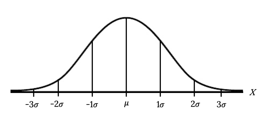
Notice that almost all the x values lie within three standard deviations of the mean. The empirical rule is also known as the 68-95-99.7 rule.
Note
Suppose x has a normal distribution with mean 50 and standard deviation 6.
- About 68% of the x values lie between –1σ = (–1)(6) = –6 and 1σ = (1)(6) = 6 of the mean 50. The values 50 – 6 = 44 and 50 + 6 = 56 are within one standard deviation of the mean 50. The z-scores are –1 and +1 for 44 and 56, respectively.
- About 95% of the x values lie between –2σ = (–2)(6) = –12 and 2σ = (2)(6) = 12. The values 50 – 12 = 38 and 50 + 12 = 62 are within two standard deviations of the mean 50. The z-scores are –2 and +2 for 38 and 62, respectively.
- About 99.7% of the x values lie between –3σ = (–3)(6) = –18 and 3σ = (3)(6) = 18 of the mean 50. The values 50 – 18 = 32 and 50 + 18 = 68 are within three standard deviations of the mean 50. The z-scores are –3 and +3 for 32 and 68, respectively.
Example
From 1984 to 1985, the mean height of 15- to 18-year-old males from Chile was 172.36 cm, and the standard deviation was 6.34 cm. Let Y = the height of 15- to 18-year-old males in 1984 to 1985. Then Y ~ N(172.36, 6.34).
Your Turn!
The scores on a college entrance exam have an approximate normal distribution with mean, µ = 52 points and a standard deviation, σ = 11 points.
- About 68% of the y values lie between what two values? These values are ________________. The z-scores are ________________, respectively.
- About 95% of the y values lie between what two values? These values are ________________. The z-scores are ________________, respectively.
- About 99.7% of the y values lie between what two values? These values are ________________. The z-scores are ________________, respectively.
Solution
- About 68% of the values lie between the values 41 and 63. The z-scores are –1 and 1, respectively.
- About 95% of the values lie between the values 30 and 74. The z-scores are –2 and 2, respectively.
- About 99.7% of the values lie between the values 19 and 85. The z-scores are –3 and 3, respectively.
Your Turn!
Suppose X has a normal distribution with mean 25 and standard deviation five. Between what values of x do 68% of the values lie?
Solution
between 20 and 30.
References
“Blood Pressure of Males and Females.” StatCrunch, 2013. Available online at http://www.statcrunch.com/5.0/viewreport.php?reportid=11960 (accessed May 14, 2013).
“The Use of Epidemiological Tools in Conflict-affected populations: Open-access educational resources for policy-makers: Calculation of z-scores.” London School of Hygiene and Tropical Medicine, 2009. Available online at http://conflict.lshtm.ac.uk/page_125.htm (accessed May 14, 2013).
“2012 College-Bound Seniors Total Group Profile Report.” CollegeBoard, 2012. Available online at http://media.collegeboard.com/digitalServices/pdf/research/TotalGroup-2012.pdf (accessed May 14, 2013).
“Digest of Education Statistics: ACT score average and standard deviations by sex and race/ethnicity and percentage of ACT test takers, by selected composite score ranges and planned fields of study: Selected years, 1995 through 2009.” National Center for Education Statistics. Available online at http://nces.ed.gov/programs/digest/d09/tables/dt09_147.asp (accessed May 14, 2013).
Data from the San Jose Mercury News.
Data from The World Almanac and Book of Facts.
“List of stadiums by capacity.” Wikipedia. Available online at https://en.wikipedia.org/wiki/List_of_stadiums_by_capacity (accessed May 14, 2013).
Data from the National Basketball Association. Available online at www.nba.com (accessed May 14, 2013).
Media Attributions
- Private: Figure 5.10 © Significant Statistics by John Morgan Russell is licensed under a CC BY-SA (Attribution ShareAlike) license
- Private: Figure 5.11 © Significant Statistics by John Morgan Russell is licensed under a CC BY-SA (Attribution ShareAlike) license
A function that defines a continuous random variable, and the likelihood of an outcome
a continuous random variable (RV) with a mean of 0 and a standard deviation of 1 which z-scores follow: X ~ N(0, 1); when X follows the standard normal distribution, it is often noted as Z ~ N(0, 1).
the linear transformation of the form z = [latex]\frac{x\text{ }–\text{ }\mu }{\sigma }[/latex]; if this transformation is applied to any normal distribution X ~ N(μ, σ) the result is the standard normal distribution Z ~ N(0,1). If this transformation is applied to any specific value x of the RV with mean μ and standard deviation σ, the result is called the z-score of x. The z-score allows us to compare data that are normally distributed but scaled differently.
Roughly 68% of values are within 1 standard deviation of the mean, roughly 95% of values are within 2 standard deviations of the mean, and 99.7% of values are within 3 standard deviations of the mean
