Chapter 2: Descriptive Statistics
Chapter 2 Practice
Bringing It Together from 2.4
Santa Clara County, CA, has approximately 27,873 Japanese Americans. Their ages are as follows:
| Age Group | Percentage of Community |
|---|---|
| 0–17 | 18.9 |
| 18–24 | 8.0 |
| 25–34 | 22.8 |
| 35–44 | 15.0 |
| 45–54 | 13.1 |
| 55–64 | 11.9 |
| 65+ | 10.3 |
- Construct a histogram of the Japanese American community in Santa Clara County, CA. The bars will not be the same width for this example. Why not? What impact does this have on the reliability of the graph?
- What percentage of the community is under age 35?
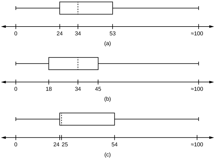
- Which box plot most resembles the information above?
Solution
- For graph, check student’s solution.
- 49.7% of the community is under the age of 35.
- Based on the information in the table, graph (a) most closely represents the data.
Bringing It Together from 2.5
Javier and Ercilia are supervisors at a shopping mall. Each was given the task of estimating the mean distance that shoppers live from the mall. They each randomly surveyed 100 shoppers. The samples yielded the following information.
| Javier | Ercilia | |
|---|---|---|
| [latex]\overline{x}[/latex] | 6.0 miles | 6.0 miles |
| [latex]s[/latex] | 4.0 miles | 7.0 miles |
- How can you determine which survey was correct?
- Explain what the difference in the results of the surveys implies about the data.
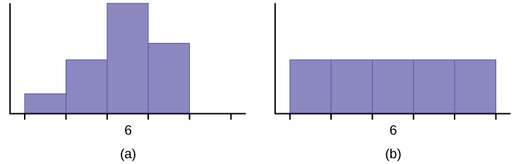
- If the two histograms depict the distribution of values for each supervisor, which one depicts Ercilia’s sample? How do you know?
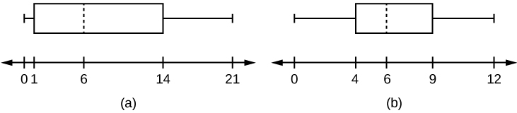
- If the two box plots depict the distribution of values for each supervisor, which one depicts Ercilia’s sample? How do you know?
Use the following information to answer the next three exercises: We are interested in the number of years students in a particular elementary statistics class have lived in California. The information in the following table is from the entire section.
| Number of years | Frequency | Number of years | Frequency |
|---|---|---|---|
| Total = 20 | |||
| 7 | 1 | 22 | 1 |
| 14 | 3 | 23 | 1 |
| 15 | 1 | 26 | 1 |
| 18 | 1 | 40 | 2 |
| 19 | 4 | 42 | 2 |
| 20 | 3 |
What is the IQR?
- 8
- 11
- 15
- 35
Solution
a
What is the mode?
- 19
- 19.5
- 14 and 20
- 22.65
Is this a sample or the entire population?
- sample
- entire population
- neither
Solution
b
Bringing It Together from 2.7
Twenty-five randomly selected students were asked the number of movies they watched the previous week. The results are as follows:
| # of movies | Frequency |
|---|---|
| 0 | 5 |
| 1 | 9 |
| 2 | 6 |
| 3 | 4 |
| 4 | 1 |
- Find the sample mean [latex]\overline{x}[/latex].
- Find the approximate sample standard deviation, s.
Solution
- 1.48
- 1.12
Forty randomly selected students were asked the number of pairs of sneakers they owned. Let X = the number of pairs of sneakers owned. The results are as follows:
| X | Frequency |
|---|---|
| 1 | 2 |
| 2 | 5 |
| 3 | 8 |
| 4 | 12 |
| 5 | 12 |
| 6 | 0 |
| 7 | 1 |
- Find the sample mean [latex]\overline{x}[/latex]
- Find the sample standard deviation, s
- Construct a histogram of the data.
- Complete the columns of the chart.
- Find the first quartile.
- Find the median.
- Find the third quartile.
- Construct a box plot of the data.
- What percent of the students owned at least five pairs?
- Find the 40th percentile.
- Find the 90th percentile.
- Construct a line graph of the data
- Construct a stemplot of the data
Following are the published weights (in pounds) of all of the team members of the San Francisco 49ers from a previous year.
177; 205; 210; 210; 232; 205; 185; 185; 178; 210; 206; 212; 184; 174; 185; 242; 188; 212; 215; 247; 241; 223; 220; 260; 245; 259; 278; 270; 280; 295; 275; 285; 290; 272; 273; 280; 285; 286; 200; 215; 185; 230; 250; 241; 190; 260; 250; 302; 265; 290; 276; 228; 265
- Organize the data from smallest to largest value.
- Find the median.
- Find the first quartile.
- Find the third quartile.
- Construct a box plot of the data.
- The middle 50% of the weights are from _______ to _______.
- If our population were all professional football players, would the above data be a sample of weights or the population of weights? Why?
- If our population included every team member who ever played for the San Francisco 49ers, would the above data be a sample of weights or the population of weights? Why?
- Assume the population was the San Francisco 49ers. Find:
- the population mean, μ.
- the population standard deviation, σ.
- the weight that is two standard deviations below the mean.
- When Steve Young, quarterback, played football, he weighed 205 pounds. How many standard deviations above or below the mean was he?
- That same year, the mean weight for the Dallas Cowboys was 240.08 pounds with a standard deviation of 44.38 pounds. Emmitt Smith weighed in at 209 pounds. With respect to his team, who was lighter, Smith or Young? How did you determine your answer?
Solution
- 174; 177; 178; 184; 185; 185; 185; 185; 188; 190; 200; 205; 205; 206; 210; 210; 210; 212; 212; 215; 215; 220; 223; 228; 230; 232; 241; 241; 242; 245; 247; 250; 250; 259; 260; 260; 265; 265; 270; 272; 273; 275; 276; 278; 280; 280; 285; 285; 286; 290; 290; 295; 302
- 241
- 205.5
- 272.5
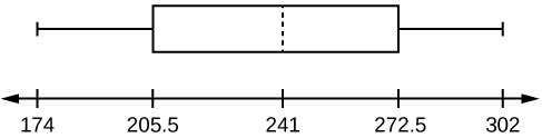
- 205.5, 272.5
- sample
- population
- 236.34
- 37.50
- 161.34
- 0.84 std. dev. below the mean
- Young
One hundred teachers attended a seminar on mathematical problem solving. The attitudes of a representative sample of 12 of the teachers were measured before and after the seminar. A positive number for change in attitude indicates that a teacher’s attitude toward math became more positive. The 12 change scores are as follows:
3 8–12 05–31–16 5–2
- What is the mean change score?
- What is the standard deviation for this population?
- What is the median change score?
- Find the change score that is 2.2 standard deviations below the mean.
Refer to [link] determine which of the following are true and which are false. Explain your solution to each part in complete sentences.
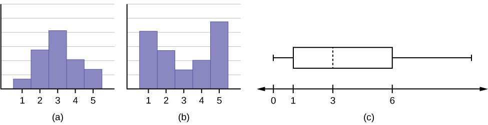
- The medians for all three graphs are the same.
- We cannot determine if any of the means for the three graphs is different.
- The standard deviation for graph b is larger than the standard deviation for graph a.
- We cannot determine if any of the third quartiles for the three graphs is different.
Solution
In a recent issue of the IEEE Spectrum, 84 engineering conferences were announced. Four conferences lasted two days. Thirty-six lasted three days. Eighteen lasted four days. Nineteen lasted five days. Four lasted six days. One lasted seven days. One lasted eight days. One lasted nine days. Let X = the length (in days) of an engineering conference.
- Organize the data in a chart.
- Find the median, the first quartile, and the third quartile.
- Find the 65th percentile.
- Find the 10th percentile.
- Construct a box plot of the data.
- The middle 50% of the conferences last from _______ days to _______ days.
- Calculate the sample mean of days of engineering conferences.
- Calculate the sample standard deviation of days of engineering conferences.
- Find the mode.
- If you were planning an engineering conference, which would you choose as the length of the conference: mean; median; or mode? Explain why you made that choice.
- Give two reasons why you think that three to five days seem to be popular lengths of engineering conferences.
A survey of enrollment at 35 community colleges across the United States yielded the following figures:
6414; 1550; 2109; 9350; 21828; 4300; 5944; 5722; 2825; 2044; 5481; 5200; 5853; 2750; 10012; 6357; 27000; 9414; 7681; 3200; 17500; 9200; 7380; 18314; 6557; 13713; 17768; 7493; 2771; 2861; 1263; 7285; 28165; 5080; 11622
- Organize the data into a chart with five intervals of equal width. Label the two columns “Enrollment” and “Frequency.”
- Construct a histogram of the data.
- If you were to build a new community college, which piece of information would be more valuable: the mode or the mean?
- Calculate the sample mean.
- Calculate the sample standard deviation.
- A school with an enrollment of 8,000 would be how many standard deviations away from the mean?
Solution
-
Enrollment Frequency 1000-5000 10 5000-10000 16 10000-15000 3 15000-20000 3 20000-25000 1 25000-30000 2 - Check student’s solution.
- mode
- 8628.74
- 6943.88
- –0.09
Use the following information to answer the next two exercises. X = the number of days per week that 100 clients use a particular exercise facility.
| x | Frequency |
|---|---|
| 0 | 3 |
| 1 | 12 |
| 2 | 33 |
| 3 | 28 |
| 4 | 11 |
| 5 | 9 |
| 6 | 4 |
The 80th percentile is _____
- 5
- 80
- 3
- 4
The number that is 1.5 standard deviations BELOW the mean is approximately _____
- 0.7
- 4.8
- –2.8
- Cannot be determined
Solution
a
Suppose that a publisher conducted a survey asking adult consumers the number of fiction paperback books they had purchased in the previous month. The results are summarized in the [link].
| # of books | Freq. | Rel. Freq. |
|---|---|---|
| 0 | 18 | |
| 1 | 24 | |
| 2 | 24 | |
| 3 | 22 | |
| 4 | 15 | |
| 5 | 10 | |
| 7 | 5 | |
| 9 | 1 |
- Are there any outliers in the data? Use an appropriate numerical test involving the IQR to identify outliers, if any, and clearly state your conclusion.
- If a data value is identified as an outlier, what should be done about it?
- Are any data values further than two standard deviations away from the mean? In some situations, statisticians may use this criteria to identify data values that are unusual, compared to the other data values. (Note that this criteria is most appropriate to use for data that is mound-shaped and symmetric, rather than for skewed data.)
- Do parts a and c of this problem give the same answer?
- Examine the shape of the data. Which part, a or c, of this question gives a more appropriate result for this data?
- Based on the shape of the data which is the most appropriate measure of center for this data: mean, median, or mode?
