
Chapter 8: Hypothesis Testing with One Sample
8.5 Additional Information and Full Hypothesis Test Examples
Learning Objectives
By the end of this section, the student should be able to:
- Conduct and interpret hypothesis tests for a single population mean, population standard deviation known.
- Conduct and interpret hypothesis tests for a single population mean, population standard deviation unknown.
- Conduct and interpret hypothesis tests for a single population proportion.
Hypothesis Tests for a Single Population Mean, Population Standard Deviation Known
- In a hypothesis test problem, you may see words such as “the level of significance is 1%.” The “1%” is the preconceived or preset α.
- The statistician setting up the hypothesis test selects the value of α to use before collecting the sample data.
- If no level of significance is given, a common standard to use is α = 0.05.
- When you calculate the p-value and draw the picture, the p-value is the area in the left tail, the right tail, or split evenly between the two tails. For this reason, we call the hypothesis test left, right, or two tailed.
- The alternative hypothesis, [latex]{H}_{a}[/latex], tells you if the test is left, right, or two-tailed. It is the key to conducting the appropriate test.
- Ha never has a symbol that contains an equal sign.
- Thinking about the meaning of the p-value: A data analyst (and anyone else) should have more confidence that he made the correct decision to reject the null hypothesis with a smaller p-value (for example, 0.001 as opposed to 0.04) even if using the 0.05 level for alpha. Similarly, for a large p-value such as 0.4, as opposed to a p-value of 0.056 (alpha = 0.05 is less than either number), a data analyst should have more confidence that she made the correct decision in not rejecting the null hypothesis. This makes the data analyst use judgment rather than mindlessly applying rules.
The following examples illustrate a left-, right-, and two-tailed test.
Example
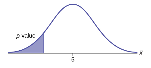
Ho: μ = 5, Ha: μ < 5
Test of a single population mean. Ha tells you the test is left-tailed. The picture of the p-value is as follows:
Your Turn!
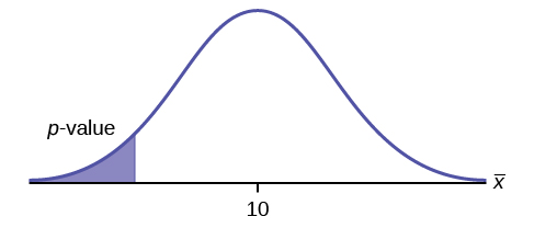
H0: μ = 10, Ha: μ < 10
Assume the p-value is 0.0935. What type of test is this? Draw the picture of the p-value.
Solution
left-tailed test
Example
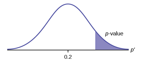
H0: p ≤ 0.2 Ha: p > 0.2
This is a test of a single population proportion. Ha tells you the test is right-tailed. The picture of the p-value is as follows:
Your Turn!
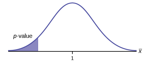
H0: μ ≤ 1, Ha: μ > 1
Assume the p-value is 0.1243. What type of test is this? Draw the picture of the p-value.
Solution
right-tailed test
Example
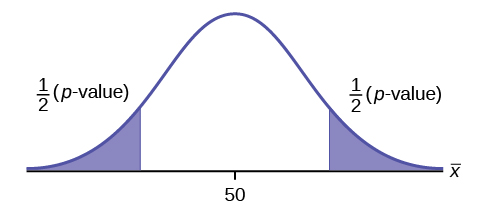
H0: p = 50 Ha: p ≠ 50
This is a test of a single population mean. Ha tells you the test is two-tailed. The picture of the p-value is as follows.
Your Turn!
H0: p = 0.5, Ha: p ≠ 0.5
Assume the p-value is 0.2564. What type of test is this? Draw the picture of the p-value.
Solution
two-tailed test
 \
\Full Hypothesis Test Examples
Example
Jeffrey, as an eight-year old, established a mean time of 16.43 seconds for swimming the 25-yard freestyle, with a standard deviation of 0.8 seconds. His dad, Frank, thought that Jeffrey could swim the 25-yard freestyle faster using goggles. Frank bought Jeffrey a new pair of expensive goggles and timed Jeffrey for 15 25-yard freestyle swims. For the 15 swims, Jeffrey’s mean time was 16 seconds. Frank thought that the goggles helped Jeffrey to swim faster than the 16.43 seconds. Conduct a hypothesis test using a preset α = 0.05. Assume that the swim times for the 25-yard freestyle are normal.
Solution
Set up the Hypothesis Test:
Since the problem is about a mean, this is a test of a single population mean.
H0: μ = 16.43 Ha: μ < 16.43
For Jeffrey to swim faster, his time will be less than 16.43 seconds. The “<” tells you this is left-tailed.
Determine the distribution needed:
Random variable: [latex]\overline{X}[/latex] = the mean time to swim the 25-yard freestyle.
Distribution for the test: [latex]\overline{X}[/latex] is normal (population standard deviation is known: σ = 0.8)
[latex]\overline{X}~N\left(\mu ,\frac{{\sigma }_{X}}{\sqrt{n}}\right)[/latex]
Therefore, [latex]\overline{X}~N\left(16.43,\frac{0.8}{\sqrt{15}}\right)[/latex]
μ = 16.43 comes from H0 and not the data. σ = 0.8, and n = 15.
Calculate the p-value using the normal distribution for a mean:
p-value = P([latex]\overline{x}[/latex] < 16) = 0.0187 where the sample mean in the problem is given as 16.
p-value = 0.0187 (This is called the actual level of significance.) The p-value is the area to the left of the sample mean is given as 16.
Graph:
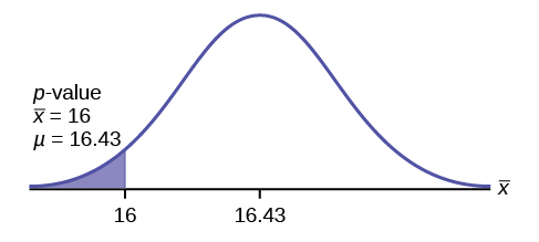
μ = 16.43 comes from H0. Our assumption is μ = 16.43.
Interpretation of the p-value: If H0 is true, there is a 0.0187 probability (1.87%)that Jeffrey’s mean time to swim the 25-yard freestyle is 16 seconds or less. Because a 1.87% chance is small, the mean time of 16 seconds or less is unlikely to have happened randomly. It is a rare event.
Compare α and the p-value:
α = 0.05 p-value = 0.0187 α > p-value
Make a decision: Since α > p-value, reject H0.
<!– CONTINUE HERE –>
This means that you reject μ = 16.43. In other words, you do not think Jeffrey swims the
25-yard freestyle in 16.43 seconds but faster with the new goggles.
Conclusion: At the 5% significance level, we conclude that Jeffrey swims faster using the new goggles. The sample data show there is sufficient evidence that Jeffrey’s mean time to swim the 25-yard freestyle is less than 16.43 seconds.
The p-value can easily be calculated.
Press STAT and arrow over to TESTS. Press 1:Z-Test. Arrow over to Stats and press ENTER. Arrow down and enter 16.43 for μ0 (null hypothesis), .8 for σ, 16 for the sample mean, and 15 for n. Arrow down to μ : (alternate hypothesis) and arrow over to < μ0. Press ENTER. Arrow down to Calculate and press ENTER. The calculator not only calculates the p-value (p = 0.0187) but it also calculates the test statistic (z-score) for the sample mean. μ < 16.43 is the alternative hypothesis. Do this set of instructions again except arrow to Draw(instead of Calculate). Press ENTER. A shaded graph appears with z = -2.08 (test statistic) and p = 0.0187 (p-value). Make sure when you use Draw that no other equations are highlighted in Y = and the plots are turned off.
When the calculator does a Z-Test, the Z-Test function finds the p-value by doing a normal probability calculation using the central limit theorem:
[latex]P\left(\overline{x}16\right)=[/latex]2nd DISTR normcdf[latex]\left(-10^99,16,16.43,0.8/\sqrt{15}\right)[/latex] .
The Type I and Type II errors for this problem are as follows:
The Type I error is to conclude that Jeffrey swims the 25-yard freestyle, on average, in
less than 16.43 seconds when, in fact, he actually swims the 25-yard freestyle, on
average, in 16.43 seconds. (Reject the null hypothesis when the null hypothesis is true.)
The Type II error is that there is no evidence to conclude that Jeffrey swims the 25-yard free-style, on average, in less than 16.43 seconds when, in fact, he actually does swim the 25-yard free-style, on average, in less than 16.43 seconds. (Do not reject the null hypothesis when the null hypothesis is false.)
Your Turn!
The mean throwing distance of a football for Marco, a high school freshman quarterback, is 40 yards, with a standard deviation of two yards. The team coach tells Marco to adjust his grip to get more distance. The coach records the distances for 20 throws. For the 20 throws, Marco’s mean distance was 45 yards. The coach thought the different grip helped Marco throw farther than 40 yards. Conduct a hypothesis test using a preset α = 0.05. Assume the throw distances for footballs are normal.
First, determine what type of test this is, set up the hypothesis test, find the p-value, sketch the graph, and state your conclusion.
Press STAT and arrow over to TESTS. Press 1:Z-Test. Arrow over to Stats and press ENTER. Arrow down and enter 40 for μ0 (null hypothesis), 2 for σ, 45 for the sample mean, and 20 for n. Arrow down to μ: (alternative hypothesis) and set it either as <, ≠, or >. Press ENTER. Arrow down to Calculate and press ENTER. The calculator not only calculates the p-value but it also calculates the test statistic (z-score) for the sample mean. Select <, ≠, or > for the alternative hypothesis. Do this set of instructions again except arrow to Draw (instead of Calculate). Press ENTER. A shaded graph appears with test statistics and p-value. Make sure when you use Draw that no other equations are highlighted in Y = and the plots are turned off.
Solution
Since the problem is about a mean, this is a test of a single population mean.
H0 : μ = 40
Ha : μ > 40
p = 0.0062

Because p < α, we reject the null hypothesis. There is sufficient evidence to suggest that the change in grip improved Marco’s throwing distance.
Historical Note ([link])
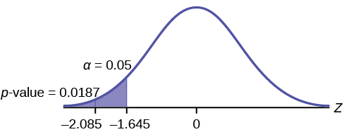
The traditional way to compare the two probabilities, α and the p-value, is to compare the critical value (z-score from α) to the test statistic (z-score from data). The calculated test statistic for the p-value is –2.08. (From the Central Limit Theorem, the test statistic formula is [latex]z=\frac{\overline{x}-{\mu }_{X}}{\left(\frac{{\sigma }_{X}}{\sqrt{n}}\right)}[/latex].)
For this problem, [latex]\overline{x}[/latex] = 16, μX = 16.43 from the null hypothesis is σX = 0.8, and n = 15.) You can find the critical value for α = 0.05 in the normal table (see 15.Tables in the Table of Contents). The z-score for an area to the left equal to 0.05 is midway between –1.65 and –1.64 (0.05 is midway between 0.0505 and 0.0495). The z-score is –1.645. Since –1.645 > –2.08 (which demonstrates that α > p-value), reject H0. Traditionally, the decision to reject or not reject was done in this way. Today, comparing the two probabilities α and the p-value is very common. For this problem, the p-value, 0.0187 is considerably smaller than α, 0.05. You can be confident about your decision to reject. The graph shows α, the p-value, and the test statistics and the critical value.
Example
A college football coach thought that his players could bench press a mean weight of 275 pounds. It is known that the standard deviation is 55 pounds. Three of his players thought that the mean weight was more than that amount. They asked 30 of their teammates for their estimated maximum lift on the bench press exercise. The data ranged from 205 pounds to 385 pounds. The actual different weights were (frequencies are in parentheses) 205(3)215(3)225(1)241(2)252(2)265(2)275(2)313(2)316(5)338(2)341(1)345(2)368(2)385(1).
Conduct a hypothesis test using a 2.5% level of significance to determine if the bench press mean is more than 275 pounds.
Solution
Set up the Hypothesis Test:
Since the problem is about a mean weight, this is a test of a single population mean.
H0: μ = 275
Ha: μ > 275
This is a right-tailed test.
Calculating the distribution needed:
Random variable: [latex]\overline{X}[/latex] = the mean weight, in pounds, lifted by the football players.
Distribution for the test: It is normal because σ is known.
[latex]\overline{X}~N\left(275,\frac{55}{\sqrt{30}}\right)[/latex]
[latex]\overline{x}=286.2[/latex] pounds (from the data).
σ = 55 pounds (Always use σ if you know it.) We assume μ = 275 pounds unless our data shows us otherwise.
Calculate the p-value using the normal distribution for a mean and using the sample mean as input (see [link] for using the data as input):
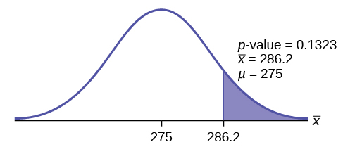
[latex]p\text{-value}=P\left(\overline{x}>286.2\right)=0.1323[/latex].
Interpretation of the p-value: If H0 is true, then there is a 0.1331 probability (13.23%) that the football players can lift a mean weight of 286.2 pounds or more. Because a 13.23% chance is large enough, a mean weight lift of 286.2 pounds or more is not a rare event.
Compare α and the p-value:
α = 0.025 p-value = 0.1323
Make a decision: Since α <p-value, do not reject H0.
Conclusion: At the 2.5% level of significance, from the sample data, there is not sufficient evidence to conclude that the true mean weight lifted is more than 275 pounds.
The p-value can easily be calculated.
Put the data and frequencies into lists. Press STAT and arrow over to TESTS. Press 1:Z-Test. Arrow over to Data and press ENTER. Arrow down and enter 275 for μ0, 55 for σ, the name of the list where you put the data, and the name of the list where you put the frequencies. Arrow down to μ: and arrow over to > μ0. Press ENTER. Arrow down to Calculate and press ENTER. The calculator not only calculates the p-value (p = 0.1331, a little different from the previous calculation—in it we used the sample mean rounded to one decimal place instead of the data) but it also calculates the test statistic (z-score) for the sample mean, the sample mean, and the sample standard deviation. μ > 275 is the alternative hypothesis. Do this set of instructions again except arrow to Draw (instead of Calculate). Press ENTER. A shaded graph appears with z = 1.112 (test statistic) and p = 0.1331 (p-value). Make sure when you use Draw that no other equations are highlighted in Y = and the plots are turned off.
Hypothesis Tests for a Single Population Mean, Population Standard Deviation Unknown
Example
Statistics students believe that the mean score on the first statistics test is 65. A statistics instructor thinks the mean score is higher than 65. He samples ten statistics students and obtains the scores 65657067666363687271. He performs a hypothesis test using a 5% level of significance. The data are assumed to be from a normal distribution.
Solution
Set up the hypothesis test:
A 5% level of significance means that α = 0.05. This is a test of a single population mean.
H0: μ = 65 Ha: μ > 65
Since the instructor thinks the average score is higher, use a “>”. The “>” means the test is right-tailed.
Determine the distribution needed:
Random variable:[latex]\overline{X}[/latex] = average score on the first statistics test.
Distribution for the test: If you read the problem carefully, you will notice that there is
no population standard deviation given. You are only given n = 10 sample data values. Notice also that the data come from a normal distribution. This means that the distribution for the test is a student’s t.
Use tdf. Therefore, the distribution for the test is t9 where n = 10 and df = 10 – 1 = 9.
Calculate the p-value using the Student’s t-distribution:
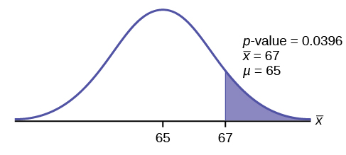
p-value = P([latex]\overline{x}[/latex] > 67) = 0.0396 where the sample mean and sample standard deviation are calculated as 67 and 3.1972 from the data.
Interpretation of the p-value: If the null hypothesis is true, then there is a 0.0396
probability (3.96%) that the sample mean is 65 or more.
Compare α and the p-value:
Since α = 0.05 and p-value = 0.0396. α > p-value.
Make a decision: Since α > p-value, reject H0.
This means you reject μ = 65. In other words, you believe the average test score is more than 65.
Conclusion: At a 5% level of significance, the sample data show sufficient evidence that the mean (average) test score is more than 65, just as the math instructor thinks.
The p-value can easily be calculated.
Put the data into a list. Press STAT and arrow over to TESTS. Press 2:T-Test. Arrow over to Data and press ENTER. Arrow down and enter 65 for μ0, the name of the list where you put the data, and 1 for Freq:. Arrow down to μ: and arrow over to > μ0. Press ENTER. Arrow down to Calculate and press ENTER. The calculator not only calculates the p-value (p = 0.0396) but it also calculates the test statistic (t-score) for the sample mean, the sample mean, and the sample standard deviation. μ > 65 is the alternative hypothesis. Do this set of instructions again except arrow to Draw (instead of Calculate). Press ENTER. A shaded graph appears with t = 1.9781 (test statistic) and p = 0.0396 (p-value). Make sure when you use Draw that no other equations are highlighted in Y = and the plots are turned off.
Your Turn!
It is believed that a stock price for a particular company will grow at a rate of 💲5 per week with a standard deviation of 💲1. An investor believes the stock won’t grow as quickly. The changes in stock price is recorded for ten weeks and are as follows: 💲4, 💲3, 💲2, 💲3, 💲1, 💲7, 💲2, 💲1, 💲1, 💲2. Perform a hypothesis test using a 5% level of significance. State the null and alternative hypotheses, find the p-value, state your conclusion, and identify the Type I and Type II errors.
Solution
H0: μ = 5
Ha: μ < 5
p = 0.0082
Because p < α, we reject the null hypothesis. There is sufficient evidence to suggest that the stock price of the company grows at a rate less than 💲5 a week.
Type I Error: To conclude that the stock price is growing slower than 💲5 a week when, in fact, the stock price is growing at 💲5 a week (reject the null hypothesis when the null hypothesis is true).
Type II Error: To conclude that the stock price is growing at a rate of 💲5 a week when, in fact, the stock price is growing slower than 💲5 a week (do not reject the null hypothesis when the null hypothesis is false).
Hypothesis Tests for a Single Population Proportion
Example
Joon believes that 50% of first-time brides in the United States are younger than their grooms. She performs a hypothesis test to determine if the percentage is the same or different from 50%. Joon samples 100 first-time brides and 53 reply that they are younger than their grooms. For the hypothesis test, she uses a 1% level of
significance.
Solution
Set up the hypothesis test:
The 1% level of significance means that α = 0.01. This is a test of a single population proportion.
H0: p = 0.50 Ha: p ≠ 0.50
The words “is the same or different from” tell you this is a two-tailed test.
Calculate the distribution needed:
Random variable: P′ = the percentage of first-time brides who are younger than their grooms.
Distribution for the test: The problem contains no mention of a mean. The
information is given in terms of percentages. Use the distribution for P′, the estimated proportion.
[latex]{P}^{\prime }~N\left(p,\sqrt{\frac{p\cdot q}{n}}\right)[/latex] Therefore, [latex]{P}^{\prime }~N\left(0.5,\sqrt{\frac{0.5\cdot 0.5}{100}}\right)[/latex]
where p = 0.50, q = 1−p = 0.50, and n = 100
Calculate the p-value using the normal distribution for proportions:
p-value = P (p′ < 0.47 or p′ > 0.53) = 0.5485
where x = 53, p′ = [latex]\frac{x}{n}\text{ = }\frac{\text{53}}{\text{100}}[/latex] = 0.53.
Interpretation of the p-value: If the null hypothesis is true, there is 0.5485 probability
(54.85%) that the sample (estimated) proportion [latex]p\text{'}[/latex] is 0.53 or more OR 0.47 or less (see
the graph in [link]).
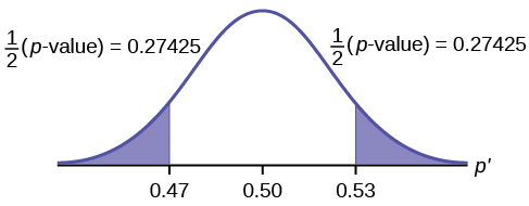
μ = p = 0.50 comes from H0, the null hypothesis.
p′ = 0.53. Since the curve is symmetrical and the test is two-tailed, the p′ for the left tail is equal to 0.50 – 0.03 = 0.47 where μ = p = 0.50. (0.03 is the difference between 0.53 and 0.50.)
Compare α and the p-value:
Since α = 0.01 and p-value = 0.5485. α < p-value.
Make a decision: Since α < p-value, you cannot reject H0.
Conclusion: At the 1% level of significance, the sample data do not show sufficient evidence that the percentage of first-time brides who are younger than their grooms is different from 50%.
The p-value can easily be calculated.
Press STAT and arrow over to TESTS. Press 5:1-PropZTest. Enter .5 for p0, 53 for x and 100 for n. Arrow down to Prop and arrow to not equals p0. Press ENTER. Arrow down to Calculate and press ENTER. The calculator calculates the p-value (p = 0.5485) and the test statistic (z-score). Prop not equals .5 is the alternate hypothesis. Do this set of instructions again except arrow to Draw (instead of Calculate). Press ENTER. A shaded graph appears with z = 0.6 (test statistic) and p = 0.5485 (p-value). Make sure when you use Draw that no other equations are highlighted in Y = and the plots are turned off.
The Type I and Type II errors are as follows:
The Type I error is to conclude that the proportion of first-time brides who are younger than their grooms is different from 50% when, in fact, the proportion is actually 50%. (Reject the null hypothesis when the null hypothesis is true).
The Type II error is there is not enough evidence to conclude that the proportion of first time brides who are younger than their grooms differs from 50% when, in fact, the proportion does differ from 50%. (Do not reject the null hypothesis when the null hypothesis is false.)
Your Turn!
A teacher believes that 85% of students in the class will want to go on a field trip to the local zoo. She performs a hypothesis test to determine if the percentage is the same or different from 85%. The teacher samples 50 students and 39 reply that they would want to go to the zoo. For the hypothesis test, use a 1% level of significance.
First, determine what type of test this is, set up the hypothesis test, find the p-value, sketch the graph, and state your conclusion.
Solution
Since the problem is about percentages, this is a test of single population proportions.
H0 : p = 0.85
Ha: p ≠ 0.85
p = 0.7554
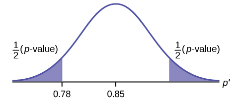
Because p > α, we fail to reject the null hypothesis. There is not sufficient evidence to suggest that the proportion of students that want to go to the zoo is not 85%.
Example
Suppose a consumer group suspects that the proportion of households that have three cell phones is 30%. A cell phone company has reason to believe that the proportion is not 30%. Before they start a big advertising campaign, they conduct a hypothesis test. Their marketing people survey 150 households with the result that 43 of the households have three cell phones.
Solution
Set up the Hypothesis Test:
H0: p = 0.30 Ha: p ≠ 0.30
Determine the distribution needed:
The random variable is P′ = proportion of households that have three cell phones.
The distribution for the hypothesis test is [latex]P\text{'}~N\left(0.30,\sqrt{\frac{\left(0.30\right)\cdot \left(0.70\right)}{150}}\right)[/latex]
a. The value that helps determine the p-value is p′. Calculate p′.
Solution
a. p′ = [latex]\frac{x}{n}[/latex] where x is the number of successes and n is the total number in the sample.
x = 43, n = 150
p′ = [latex]\frac{\text{43}}{\text{150}}[/latex]
b. What is a success for this problem?
Solution
b. A success is having three cell phones in a household.
c. What is the level of significance?
Solution
c. The level of significance is the preset α. Since α is not given, assume that α = 0.05.
d. Draw the graph for this problem. Draw the horizontal axis. Label and shade appropriately.
Calculate the p-value.
Solution
d. p-value = 0.7216
e. Make a decision. _____________(Reject/Do not reject) H0 because____________.
Solution
e. Assuming that α = 0.05, α < p-value. The decision is do not reject H0 because there is not sufficient evidence to conclude that the proportion of households that have three cell phones is not 30%.
Your Turn!
Marketers believe that 92% of adults in the United States own a cell phone. A cell phone manufacturer believes that number is actually lower. 200 American adults are surveyed, of which, 174 report having cell phones. Use a 5% level of significance. State the null and alternative hypothesis, find the p-value, state your conclusion, and identify the Type I and Type II errors.
Solution
H0: p = 0.92
Ha: p < 0.92
p-value = 0.0046
Because p < 0.05, we reject the null hypothesis. There is sufficient evidence to conclude that fewer than 92% of American adults own cell phones.
Type I Error: To conclude that fewer than 92% of American adults own cell phones when, in fact, 92% of American adults do own cell phones (reject the null hypothesis when the null hypothesis is true).
Type II Error: To conclude that 92% of American adults own cell phones when, in fact, fewer than 92% of American adults own cell phones (do not reject the null hypothesis when the null hypothesis is false).
The next example is a poem written by a statistics student named Nicole Hart. The solution to the problem follows the poem. Notice that the hypothesis test is for a single population proportion. This means that the null and alternate hypotheses use the parameter p. The distribution for the test is normal. The estimated proportion p′ is the proportion of fleas killed to the total fleas found on Fido. This is sample information. The problem gives a preconceived α = 0.01, for comparison, and a 95% confidence interval computation. The poem is clever and humorous, so please enjoy it!
Example
My dog has so many fleas, they do not come off with ease. As for shampoo, I have tried many types, even one called Bubble Hype, which only killed 25% of the fleas, unfortunately I was not pleased. I’ve used all kinds of soap, until I had given up hope, one day I saw an ad that put me in awe. A shampoo used for dogs called GOOD ENOUGH to Clean a Hog guaranteed to kill more fleas. I gave Fido a bath and after doing the math his number of fleas started dropping by 3’s! Before his shampoo I counted 42. At the end of his bath, I redid the math and the new shampoo had killed 17 fleas. So now I am pleased.
Now it is time for you to have some fun with the level of significance being .01, you must help me figure out use the new shampoo or go without?
Solution
Set up the hypothesis test:
H0: p ≤ 0.25 Ha: p > 0.25
Determine the distribution needed:
In words, CLEARLY state what your random variable [latex]\overline{X}[/latex] or P′ represents.
P′ = The proportion of fleas that are killed by the new shampoo
State the distribution to use for the test.
Normal:[latex]N\left(0.25,\sqrt{\frac{\left(0.25\right)\left(1-0.25\right)}{42}}\right)[/latex]
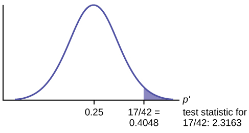
Test Statistic: z = 2.3163
Calculate the p-value using the normal distribution for proportions:
p-value = 0.0103
In one to two complete sentences, explain what the p-value means for this problem.
If the null hypothesis is true (the proportion is 0.25), then there is a 0.0103 probability that the sample (estimated) proportion is 0.4048 [latex]\left(\frac{17}{42}\right)[/latex] or more.
Use the previous information to sketch a picture of this situation. CLEARLY, label and scale the horizontal axis and shade the region(s) corresponding to the p-value.
Compare α and the p-value:
Indicate the correct decision (“reject” or “do not reject” the null hypothesis), the reason for it, and write an appropriate conclusion, using complete sentences.
| alpha | decision | reason for decision |
|---|---|---|
| 0.01 | Do not reject [latex]{H}_{0}[/latex] | α < p-value |
Conclusion: At the 1% level of significance, the sample data do not show sufficient evidence that the percentage of fleas that are killed by the new shampoo is more than 25%.
Construct a 95% confidence interval for the true mean or proportion. Include a sketch of the graph of the situation.
Label the point estimate and the lower and upper bounds of the confidence interval.
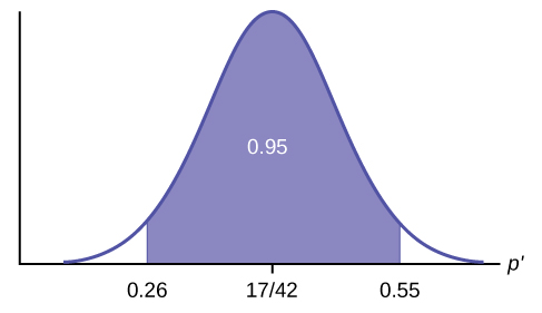
Confidence Interval: (0.26,0.55) We are 95% confident that the true population proportion p of fleas that are killed by the new shampoo is between 26% and 55%.
Note
This test result is not very definitive since the p-value is very close to alpha. In reality, one would probably do more tests by giving the dog another bath after the fleas have had a chance to return.
Example
The National Institute of Standards and Technology provides exact data on conductivity properties of materials. Following are conductivity measurements for 11 randomly selected pieces of a particular type of glass.
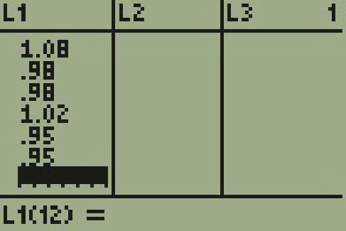
1.11; 1.07; 1.11; 1.07; 1.12; 1.08; .98; .98 1.02; .95; .95
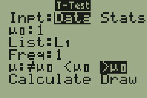
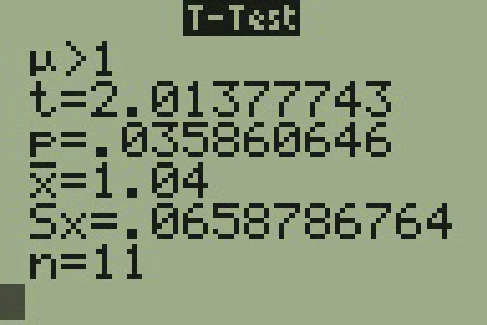
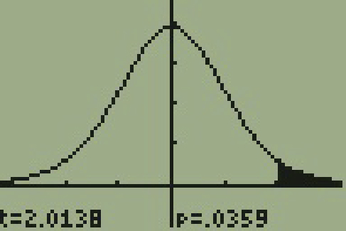
Is there convincing evidence that the average conductivity of this type of glass is greater than one? Use a significance level of 0.05. Assume the population is normal.
Solution
Let’s follow a four-step process to answer this statistical question.
State the Question: We need to determine if, at a 0.05 significance level, the average conductivity of the selected glass is greater than one. Our hypotheses will be
Do the calculations: We will input the sample data into the TI-83 as follows.
Example
In a study of 420,019 cell phone users, 172 of the subjects developed brain cancer. Test the claim that cell phone users developed brain cancer at a greater rate than that for non-cell phone users (the rate of brain cancer for non-cell phone users is 0.0340%). Since this is a critical issue, use a 0.005 significance level. Explain why the significance level should be so low in terms of a Type I error.
Solution
We will follow the four-step process.
- We need to conduct a hypothesis test on the claimed cancer rate. Our hypotheses will be
- H0: p ≤ 0.00034
- Ha: p > 0.00034
If we commit a Type I error, we are essentially accepting a false claim. Since the claim describes cancer-causing environments, we want to minimize the chances of incorrectly identifying causes of cancer.
- We will be testing a sample proportion with x = 172 and n = 420,019. The sample is sufficiently large because we have np = 420,019(0.00034) = 142.8, nq = 420,019(0.99966) = 419,876.2, two independent outcomes, and a fixed probability of success p = 0.00034. Thus we will be able to generalize our results to the population.
- The associated TI results are


- Since the p-value = 0.0073 is greater than our alpha value = 0.005, we cannot reject the null. Therefore, we conclude that there is not enough evidence to support the claim of higher brain cancer rates for the cell phone users.
Your Turn
According to the US Census there are approximately 268,608,618 residents aged 12 and older. Statistics from the Rape, Abuse, and Incest National Network indicate that, on average, 207,754 rapes occur each year (male and female) for persons aged 12 and older. This translates into a percentage of sexual assaults of 0.078%. In Daviess County, KY, there were reported 11 rapes for a population of 37,937. Conduct an appropriate hypothesis test to determine if there is a statistically significant difference between the local sexual assault percentage and the national sexual assault percentage. Use a significance level of 0.01.
Solution
We will follow the four-step plan.
- We need to test whether the proportion of sexual assaults in Daviess County, KY is significantly different from the national average.
- Since we are presented with proportions, we will use a one-proportion z-test. The hypotheses for the test will be
- H0: p = 0.00078
- Ha: p ≠ 0.00078
- The following screenshots display the summary statistics from the hypothesis test.

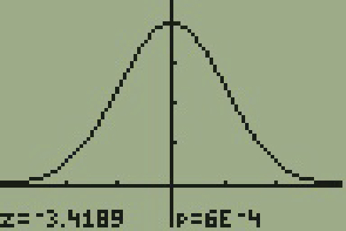
- Since the p-value, p = 0.00063, is less than the alpha level of 0.01, the sample data indicates that we should reject the null hypothesis. In conclusion, the sample data support the claim that the proportion of sexual assaults in Daviess County, Kentucky is different from the national average proportion.
References
Data from Amit Schitai. Director of Instructional Technology and Distance Learning. LBCC.
Data from Bloomberg Businessweek. Available online at http://www.businessweek.com/news/2011-
09-15/nyc-smoking-rate-falls-to-record-low-of-14-bloomberg-says.html.
Data from energy.gov. Available online at http://energy.gov (accessed June 27. 2013).
Data from Gallup®. Available online at www.gallup.com (accessed June 27, 2013).
Data from Growing by Degrees by Allen and Seaman.
Data from La Leche League International. Available online at http://www.lalecheleague.org/Law/BAFeb01.html.
Data from the American Automobile Association. Available online at www.aaa.com (accessed June 27, 2013).
Data from the American Library Association. Available online at www.ala.org (accessed June 27, 2013).
Data from the Bureau of Labor Statistics. Available online at http://www.bls.gov/oes/current/oes291111.htm.
Data from the Centers for Disease Control and Prevention. Available online at www.cdc.gov (accessed June 27, 2013)
Data from the U.S. Census Bureau, available online at http://quickfacts.census.gov/qfd/states/00000.html (accessed June 27, 2013).
Data from the United States Census Bureau. Available online at http://www.census.gov/hhes/socdemo/language/.
Data from Toastmasters International. Available online at http://toastmasters.org/artisan/detail.asp?CategoryID=1&SubCategoryID=10&ArticleID=429&Page=1.
Data from Weather Underground. Available online at www.wunderground.com (accessed June 27, 2013).
Federal Bureau of Investigations. “Uniform Crime Reports and Index of Crime in Daviess in the State of Kentucky enforced by Daviess County from 1985 to 2005.” Available online at http://www.disastercenter.com/kentucky/crime/3868.htm (accessed June 27, 2013).
“Foothill-De Anza Community College District.” De Anza College, Winter 2006. Available online at http://research.fhda.edu/factbook/DAdemofs/Fact_sheet_da_2006w.pdf.
Johansen, C., J. Boice, Jr., J. McLaughlin, J. Olsen. “Cellular Telephones and Cancer—a Nationwide Cohort Study in Denmark.” Institute of Cancer Epidemiology and the Danish Cancer Society, 93(3):203-7. Available online at http://www.ncbi.nlm.nih.gov/pubmed/11158188 (accessed June 27, 2013).
Rape, Abuse & Incest National Network. “How often does sexual assault occur?” RAINN, 2009. Available online at http://www.rainn.org/get-information/statistics/frequency-of-sexual-assault (accessed June 27, 2013).
Given a random variable (RV) with known mean [latex]\mu[/latex] and known standard deviation σ. We are sampling with size n and we are interested in two new RVs - the sample mean, [latex]\overline{X}[/latex], and the sample sum, [latex]\Sigma X[/latex].
If the size n of the sample is sufficiently large, then [latex]\overline{X}~N\left(\mu \text{,}\frac{\sigma }{\sqrt{n}}\right)[/latex] and [latex]\Sigma X~N\left(n\mu ,\sqrt{n}\sigma \right)[/latex]. If the size n of the sample is sufficiently large, then the distribution of the sample means and the distribution of the sample sums will approximate a normal distribution regardless of the shape of the population. The mean of the sample means will equal the population mean and the mean of the sample sums will equal n times the population mean. The standard deviation of the distribution of the sample means, [latex]\frac{\sigma }{\sqrt{n}}[/latex], is called the standard error of the mean.