Chapter 6: The Normal Distribution and The Central Limit Theorem
6.4 The Central Limit Theorem for Sums
Learning Objectives
By the end of this section, the student should be able to:
- Recognize characteristics of the Central Limit Theorem for the Sums
- Apply and interpret the Central Limit Theorem for the Sums and use it to solve real-world applications.
Suppose X is a random variable with a distribution that may be known or unknown (it can be any distribution) and suppose:
- μX = the mean of Χ
- σΧ = the standard deviation of X
If you draw random samples of size n, then as n increases, the random variable ΣX consisting of sums tends to be normally distributed and ΣΧ ~ N((n)(μΧ), ([latex]\sqrt{n}[/latex])(σΧ)).
The central limit theorem for sums says that if you keep drawing larger and larger samples and taking their sums, the sums form their own normal distribution (the sampling distribution), which approaches a normal distribution as the sample size increases. The normal distribution has a mean equal to the original mean multiplied by the sample size and a standard deviation equal to the original standard deviation multiplied by the square root of the sample size.
The random variable ΣX has the following z-score associated with it:
- Σx is one sum.
- [latex]z\text{ = }\frac{\Sigma x–\left(n\right)\left({\mu }_{X}\right)}{\left(\sqrt{n}\right)\left({\sigma }_{X}\right)}[/latex]
- (n)(μX) = the mean of ΣX
- [latex]\left(\sqrt{n}\right)\left({\sigma }_{X}\right)[/latex] = standard deviation of [latex]\Sigma X[/latex]
Using the TI-83, 83+, 84, 84+ Calculator
To find probabilities for sums on the calculator, follow these steps.
2nd DISTR
2:normalcdf()
normalcdf(lower value of the area, upper value of the area, (n)(mean), ([latex]\sqrt{n}[/latex])(standard deviation))
where:
- mean is the mean of the original distribution
- standard deviation is the standard deviation of the original distribution
- sample size = n
Example
An unknown distribution has a mean of 90 and a standard deviation of 15. A sample of size 80 is drawn randomly from the population.
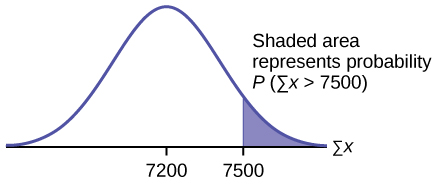
- Find the probability that the sum of the 80 values (or the total of the 80 values) is more than 7,500.
- Find the sum that is 1.5 standard deviations above the mean of the sums.
Solution
Let X = one value from the original unknown population. The probability question asks you to find a probability for the sum (or total of) 80 values.
ΣX = the sum or total of 80 values. Since μX = 90, σX = 15, and n = 80, [latex]\Sigma X[/latex] ~ N((80)(90),
([latex]\sqrt{\text{80}}[/latex])(15))
- mean of the sums = (n)(μX) = (80)(90) = 7,200
- standard deviation of the sums = [latex]\text{(}\sqrt{n}\text{)(}{\sigma }_{X}\text{) = (}\sqrt{\text{80}}\text{)}[/latex](15)
- sum of 80 values = Σx = 7,500
1. Find P(Σx > 7,500)
P(Σx > 7,500) = 0.0127
normalcdf(lower value, upper value, mean of sums, stdev of sums)
The parameter list is abbreviated(lower, upper, (n)(μX, [latex]\left(\sqrt{n}\right)[/latex](σX))
normalcdf (7500,1E99,(80)(90),[latex]\left(\sqrt{80}\right)[/latex](15)) = 0.0127
2. Find Σx where z = 1.5.
Σx = (n)(μX) + (z)[latex]\left(\sqrt{n}\right)[/latex](σΧ) = (80)(90) + (1.5)([latex]\sqrt{80}[/latex])(15) = 7,401.2
Your Turn!
An unknown distribution has a mean of 45 and a standard deviation of eight. A sample size of 50 is drawn randomly from the population. Find the probability that the sum of the 50 values is more than 2,400.
Solution
0.0040
Using the TI-83, 83+, 84, 84+ Calculator
To find percentiles for sums on the calculator, follow these steps.
2nd DIStR
3:invNorm()
k = invNorm (area to the left of k, (n)(mean), [latex]\text{(}\sqrt{n}\right)[/latex](standard deviation))
where:
- k is the kth percentile
- mean is the mean of the original distribution
- standard deviation is the standard deviation of the original distribution
- sample size = n
Example
In an October 29, 2012, study reported on the Flurry Blog, the mean age of tablet users is 34 years. Suppose the standard deviation is 15 years. The sample size is 50.
- What are the mean and standard deviation for the sum of the ages of tablet users? What is the distribution?
- Find the probability that the sum of the ages is between 1,500 and 1,800 years.
- Find the 80th percentile for the sum of the 50 ages.
Solution
- μΣx = nμx = 50(34) = 1,700 and σΣx = [latex]\sqrt{n}[/latex]σx = [latex]\left(\sqrt{\text{50}}\text{ )}[/latex](15) = 106.01
The distribution is normal for sums by the central limit theorem. - P(1500 < Σx < 1800) =
normalcdf(1,500, 1,800, (50)(34), [latex]\left(\sqrt{\text{50}}\text{ )}[/latex](15)) = 0.7974 - Let k = the 80th percentile.
k =invNorm(0.80,(50)(34),[latex]\left(\sqrt{\text{50}}\text{ )}[/latex](15)) = 1,789.3
Your Turn!
In an October 29, 2012, study reported on the Flurry Blog, the mean age of tablet users is 35 years. Suppose the standard deviation is ten years. The sample size is 39.
- What are the mean and standard deviation for the sum of the ages of tablet users? What is the distribution?
- Find the probability that the sum of the ages is between 1,400 and 1,500 years.
- Find the 90th percentile for the sum of the 39 ages.
Solution
- μΣx = nμx = 1,365 and σΣx = [latex]\sqrt{n}{\sigma }_{x}[/latex] = 62.4
The distribution is normal for sums by the central limit theorem. - P(1400 < Σx < 1500) =
normalcdf(1400,1500,(39)(35),([latex]\sqrt{39}[/latex])(10)) = 0.2723 - Let k = the 90th percentile. k =
invNorm(0.90,(39)(35),([latex]\sqrt{39}[/latex])(10)) = 1445.0
Example
The mean number of minutes for app engagement by a tablet user is 8.2 minutes. Suppose the standard deviation is one minute. Take a sample of size 70.
- What are the mean and standard deviation for the sums?
- Find the 95th percentile for the sum of the sample. Interpret this value in a complete sentence.
- Find the probability that the sum of the sample is at least ten hours.
Solution
- μΣx = nμx = 70(8.2) = 574 minutes and σΣx = [latex]\left(\sqrt{n}\right)\left({\sigma }_{x}\right)[/latex] = [latex]\left(\sqrt{\text{70}}\text{ )}[/latex](1) = 8.37 minutes
- Let k = the 95th percentile.
k = invNorm(0.95,(70)(8.2),[latex]\left(\sqrt{\text{70}}\text{)}[/latex](1)) = 587.76 minutes. Ninety five percent of the app engagement times are at most 587.76 minutes. - ten hours = 600 minutes
P(Σx ≥ 600) =normalcdf(600,E99,(70)(8.2),[latex]\left(\sqrt{\text{70}}\text{)}[/latex](1)) = 0.0009
Your Turn!
The mean number of minutes for app engagement by a tablet user is 8.2 minutes. Suppose the standard deviation is one minute. Take a sample size of 70.
- What is the probability that the sum of the sample is between seven hours and ten hours? What does this mean in context of the problem?
- Find the 84th and 16th percentiles for the sum of the sample. Interpret these values in context.
Solution
- 7 hours = 420 minutes
10 hours = 600 minutesnormalcdf[latex]P\left(420\le \Sigma x\le 600\right)=normalcdf\left(420,600,\left(70\right)\left(8.2\right),\sqrt{70}\left(1\right)\right)=0.9991[/latex]This means that for these sample sums, there is a 99.9% chance that the sums of usage minutes will be between 420 minutes and 600 minutes.
- [latex]invNorm\left(0.84,\left(70\right)\left(8.2\right),\sqrt{70}\left(1\right)\right)=582.32[/latex]
[latex]invNorm\left(0.16,\left(70\right)\left(8.2\right),\sqrt{70}\left(1\right)\right)=565.68[/latex]
Since 84% of the app engagement times are at most 582.32 minutes and 16% of the app engagement times are at most 565.68 minutes, we may state that 68% of the app engagement times are between 565.68 minutes and 582.32 minutes.
Note
It is important for you to understand when to use the central limit theorem and when to differentiate between the CLT for the Mean versus the CLT for the Sum (or Total). If you are being asked to find the probability of the mean, use the clt for the mean, but if you are being asked to find the probability of a sum or total, use the clt for sums. This also applies to percentiles for means and sums.
Example
A study involving stress is conducted among the students on a college campus. The stress scores follow a uniform distribution with the lowest stress score equal to one and the highest equal to five. Using a sample of 75 students. Find:
- The probability that the mean stress score for the 75 students is less than two.
- The 90th percentile for the mean stress score for the 75 students.
- The probability that the total of the 75 stress scores is less than 200.
- The 90th percentile for the total stress score for the 75 students.
Let X = one stress score. Problems 1 and 2 ask you to find a probability or a percentile for a mean. Problems 3 and 4 ask you to find a probability or a percentile for a total or sum.
The sample size, n, is equal to 75. Since the individual stress scores follow a uniform distribution, X ~ U(1, 5) where a = 1 and b = 5.
μX = [latex]\frac{a+b}{2}[/latex] = [latex]\frac{\text{1 + 5}}{2}[/latex] = 3
σX = [latex]\sqrt{\frac{{\left(b–a\right)}^{2}}{12}}[/latex] = [latex]\sqrt{\frac{{(5-1)}^2}{12}}[/latex] = 1.15
For problems 1 and 2., let [latex]\overline{X}[/latex] = the mean stress score for the 75 students. Then, [latex]\overline{X}[/latex] ∼ N [latex]\left(\text{3, }\frac{\text{1}\text{.15}}{\sqrt{\text{75}}}\right)[/latex] where n = 75.
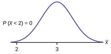
a. Find P([latex]\overline{x}[/latex] < 2).
Solution
P([latex]\overline{x}[/latex] < 2) = 0
The probability that the mean stress score is less than two is about zero.
normalcdf[latex]\left(\text{1,2,3,}\frac{\text{1}\text{.15}}{\sqrt{\text{75}}}\right)[/latex] = 0
Reminder: The smallest stress score is one.
b. Find the 90th percentile for the mean of 75 stress scores. Draw a graph.
Solution
Let k = the 90th percentile.
Find k, where P([latex]\overline{x}[/latex] < k) = 0.90.
k = 3.2
This is a normal distribution curve. The peak of the curve coincides with the point 3 on the horizontal axis. A point, k, is labeled to the right of 3. A vertical line extends from k to the curve. The area under the curve to the left of k is shaded. The shaded area shows that P(x-bar < k) = 0.90
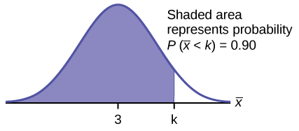
The 90th percentile for the mean of 75 scores is about 3.2. This tells us that 90% of all the means of 75 stress scores are at most 3.2, and that 10% are at least 3.2.
invNorm[latex]\left(\text{0}\text{.90,3,}\frac{1.15}{\sqrt{75}}\right)[/latex] = 3.2
For problems 3 and 4, let ΣX = the sum of the 75 stress scores. Then, ΣX ~ N[(75)(3),[latex]\left(\sqrt{75}\right)[/latex](1.15)]
c. Find P(Σx < 200). Draw the graph.
Solution
The mean of the sum of 75 stress scores is (75)(3) = 225
The standard deviation of the sum of 75 stress scores is [latex]\left(\sqrt{75}\right)[/latex](1.15) = 9.96
P(Σx < 200) = 0
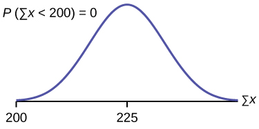
The probability that the total of 75 scores is less than 200 is about zero.
normalcdf (75,200,(75)(3),[latex]\left(\sqrt{75}\right)[/latex](1.15)).
Reminder: The smallest total of 75 stress scores is 75, because the smallest single score is one.
d. Find the 90th percentile for the total of 75 stress scores. Draw a graph.
Solution
Let k = the 90th percentile.
Find k where P(Σx < k) = 0.90.
k = 237.8
This is a normal distribution curve. The peak of the curve coincides with the point 225 on the horizontal axis. A point, k, is labeled to the right of 225. A vertical line extends from k to the curve. The area under the curve to the left of k is shaded. The shaded area shows that P(sum of x < k) = 0.90
invNorm(0.90,(75)(3),[latex]\left(\sqrt{75}\right)[/latex](1.15)) = 237.8
Example
In the United States, someone is sexually assaulted every two minutes, on average, according to a number of studies. Suppose the standard deviation is 0.5 minutes and the sample size is 100.
- Find the median, the first quartile, and the third quartile for the sample mean time of sexual assaults in the United States.
- Find the median, the first quartile, and the third quartile for the sum of sample times of sexual assaults in the United States.
- Find the probability that a sexual assault occurs on the average between 1.75 and 1.85 minutes.
- Find the value that is two standard deviations above the sample mean.
- Find the IQR for the sum of the sample times.
Solution
- We have μx = μ = 2 and σx = [latex]\frac{\sigma }{\sqrt{n}}[/latex] = [latex]\frac{0.5}{10}[/latex] = 0.05. Therefore:
- 50th percentile = μx = μ = 2
- 25th percentile = invNorm(0.25,2,0.05) = 1.97
- 75th percentile = invNorm(0.75,2,0.05) = 2.03
- We have μΣx = n(μx) = 100(2) = 200 and σμx = [latex]\sqrt{n}[/latex](σx) = 10(0.5) = 5. Therefore
- 50th percentile = μΣx = n(μx) = 100(2) = 200
- 25th percentile = invNorm(0.25,200,5) = 196.63
- 75th percentile = invNorm(0.75,200,5) = 203.37
- P(1.75 < [latex]\overline{x}[/latex] < 1.85) =
normalcdf(1.75,1.85,2,0.05) = 0.0013 - Using the z-score equation, [latex]z\text{ = }\frac{\overline{x}–{\mu }_{\overline{x}}}{{\sigma }_{\overline{x}}}[/latex], and solving for x, we have x = 2(0.05) + 2 = 2.1
- The IQR is 75th percentile – 25th percentile = 203.37 – 196.63 = 6.74
Your Turn!
A study was done about violence against prostitutes and the symptoms of the posttraumatic stress that they developed. The age range of the prostitutes was 14 to 61. The mean age was 30.9 years with a standard deviation of nine years.
- In a sample of 25 prostitutes, what is the probability that the mean age of the prostitutes is less than 35?
- Is it likely that the mean age of the sample group could be more than 50 years? Interpret the results.
- In a sample of 49 prostitutes, what is the probability that the sum of the ages is no less than 1,600?
- Is it likely that the sum of the ages of the 49 prostitutes is at most 1,595? Interpret the results.
- Find the 95th percentile for the sample mean age of 65 prostitutes. Interpret the results.
- Find the 90th percentile for the sum of the ages of 65 prostitutes. Interpret the results.
Solution
- P([latex]\overline{x}[/latex] < 35) =
normalcdf(-1E99,35,30.9,1.8) = 0.9886 - P([latex]\overline{x}[/latex] > 50) =
normalcdf(50, 1E99,30.9,1.8) ≈ 0. For this sample group, it is almost impossible for the group’s average age to be more than 50. However, it is still possible for an individual in this group to have an age greater than 50. - P(Σx ≥ 1,600) =
normalcdf(1600, 1E99,1514.10,63) = 0.0864 - P(Σx ≤ 1,595) =
normalcdf(-1E99, 1595, 1514.10, 63) = 0.9005. This means that there is a 90% chance that the sum of the ages for the sample group n = 49 is at most 1595. - The 95th percentile =
invNorm(0.95,30.9,1.1) = 32.7. This indicates that 95% of the prostitutes in the sample of 65 are younger than 32.7 years, on average. - The 90th percentile =
invNorm(0.90,2008.5,72.56) = 2101.5. This indicates that 90% of the prostitutes in the sample of 65 have a sum of ages less than 2,101.5 years.
References
Farago, Peter. “The Truth About Cats and Dogs: Smartphone vs Tablet Usage Differences.” The Flurry Blog, October 29, 2012. Available online at https://www.flurry.com/blog (accessed May 17, 2013).
