Chapter 5: Continuous Random Variables
Chapter 5 Review
5.1 Review
The probability density function (pdf) is used to describe probabilities for continuous random variables. The area under the density curve between two points corresponds to the probability that the variable falls between those two values. In other words, the area under the density curve between points a and b is equal to P(a < x < b). The cumulative distribution function (cdf) gives the probability as an area. If X is a continuous random variable, the probability density function (pdf), f(x), is used to draw the graph of the probability distribution. The total area under the graph of f(x) is one. The area under the graph of f(x) and between values a and b gives the probability P(a < x < b).
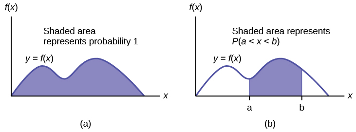
The cumulative distribution function (cdf) of X is defined by P (X ≤ x). It is a function of x that gives the probability that the random variable is less than or equal to x.
Formula Review
Probability density function (pdf) f(x):
- f(x) ≥ 0
- The total area under the curve f(x) is one.
Cumulative distribution function (cdf): P(X ≤ x)
5.2 Review
If X has a uniform distribution where a < x < b or a ≤ x ≤ b, then X takes on values between a and b (may include a and b). All values x are equally likely. We write X ∼ U(a, b). The mean of X is [latex]\mu =\frac{a+b}{2}[/latex]. The standard deviation of X is [latex]\sigma =\sqrt{\frac{{\left(b-a\right)}^{2}}{12}}[/latex]. The probability density function of X is [latex]f\left(x\right)=\frac{1}{b-a}[/latex] for a ≤ x ≤ b. The cumulative distribution function of X is P(X ≤ x) = [latex]\frac{x-a}{b-a}[/latex]. X is continuous.
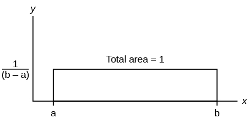
The probability P(c < X < d) may be found by computing the area under f(x), between c and d. Since the corresponding area is a rectangle, the area may be found simply by multiplying the width and the height.
Formula Review
X = a real number between a and b (in some instances, X can take on the values a and b). a = smallest X; b = largest X
X ~ U (a, b)
The mean is [latex]\mu =\frac{a+b}{2}[/latex]
The standard deviation is [latex]\sigma =\sqrt{\frac{{\left(b\text{ – }a\right)}^{2}}{12}}[/latex]
Probability density function: [latex]f\left(x\right)=\frac{1}{b-a}[/latex] for [latex]a\le X\le b[/latex]
Area to the Left of x:P(X < x) = (x – a)[latex]\left(\frac{1}{b-a}\right)[/latex]
Area to the Right of x:P(X > x) = (b – x)[latex]\left(\frac{1}{b-a}\right)[/latex]
Area Between c and d:P(c < x < d) = (base)(height) = (d – c)[latex]\left(\frac{1}{b-a}\right)[/latex]
Uniform: X ~ U(a, b) where a < x < b
- pdf: [latex]f\left(x\right)=\frac{1}{b-a}[/latex]
for a ≤ x ≤ b - cdf: P(X ≤ x) = [latex]\frac{x-a}{b-a}[/latex]
- mean µ = [latex]\frac{a+b}{2}[/latex]
- standard deviation σ [latex]=\sqrt{\frac{{\left(b-a\right)}^{2}}{12}}[/latex]
- P(c < X < d) = (d – c)[latex]\left(\frac{1}{b–a}\right)[/latex]
5.3 Review
If X has an exponential distribution with mean μ, then the decay parameter is m = [latex]\frac{1}{\mu }[/latex], and we write X ∼ Exp(m) where x ≥ 0 and m > 0. The probability density function of X is f(x) = me-mx (or equivalently [latex]f\left(x\right)=\frac{1}{\mu }{e}^{-x/\mu }[/latex]). The cumulative distribution function of X is P(X ≤ x) = 1 – e–mx.
The exponential distribution has the memoryless property, which says that future probabilities do not depend on any past information. Mathematically, it says that P(X > x + k|X > x) = P(X > k).
If T represents the waiting time between events, and if T ∼ Exp(λ), then the number of events X per unit time follows the Poisson distribution with mean λ. The probability density function of PX is [latex]\left(X=k\right)=\frac{{\lambda }^{k}{e}^{-k}}{k!}[/latex]. This may be computed using a TI-83, 83+, 84, 84+ calculator with the command poissonpdf(λ, k). The cumulative distribution function P(X ≤ k) may be computed using the TI-83, 83+,84, 84+ calculator with the command poissoncdf(λ, k).
Formula Review
Exponential: X ~ Exp(m) where m = the decay parameter
- pdf: f(x) = me(–mx) where x ≥ 0 and m > 0
- cdf: P(X ≤ x) = 1 – e(–mx)
- mean µ = [latex]\frac{1}{m}[/latex]
- standard deviation σ = µ
- percentile k: k = [latex]\frac{ln\left(1-AreaToTheLeftOfk\right)}{\left(-m\right)}[/latex]
- Additionally
- P(X > x) = e(–mx)
- P(a < X < b) = e(–ma) – e(–mb)
- Memoryless Property: P(X > x + k|X > x) = P (X > k)
- Poisson probability: [latex]P\left(X=k\right)=\frac{{\lambda}^{k}{e}^{-k}}{k!}[/latex] with mean λ
- k! = k*(k-1)*(k-2)*(k-3)…3*2*1
