Chapter 10: Linear Regression and Correlation
Chapter 10 Review
Chapter Review from 10.1
The most basic type of association is a linear association. This type of relationship can be defined algebraically by the equations used, numerically with actual or predicted data values, or graphically from a plotted curve. (Lines are classified as straight curves.) Algebraically, a linear equation typically takes the form y = mx + b, where m and b are constants, x is the independent variable, y is the dependent variable. In a statistical context, a linear equation is written in the form y = a + bx, where a and b are the constants. This form is used to help readers distinguish the statistical context from the algebraic context. In the equation y = a + bx, the constant b that multiplies the x variable (b is called a coefficient) is called the slope. The slope describes the rate of change between the independent and dependent variables; in other words, the rate of change describes the change that occurs in the dependent variable as the independent variable is changed. In the equation y = a + bx, the constant a is called the y-intercept. Graphically, the y-intercept is the y coordinate of the point where the graph of the line crosses the y axis. At this point x = 0.
The slope of a line is a value that describes the rate of change between the independent and dependent variables. The slope tells us how the dependent variable (y) changes for every one unit increase in the independent (x) variable, on average. The y-intercept is used to describe the dependent variable when the independent variable equals zero. Graphically, the slope is represented by three line types in elementary statistics.
Formula Review
y = a + bx where a is the y-intercept and b is the slope. The variable x is the independent variable and y is the dependent variable.
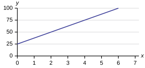
Use the following information to answer the next three exercises. A vacation resort rents SCUBA equipment to certified divers. The resort charges an up-front fee of 💲25 and another fee of 💲12.50 an hour.
What are the dependent and independent variables?
Solution
dependent variable: fee amount; independent variable: time
Find the equation that expresses the total fee in terms of the number of hours the equipment is rented.
Graph the equation from [link].
Solution
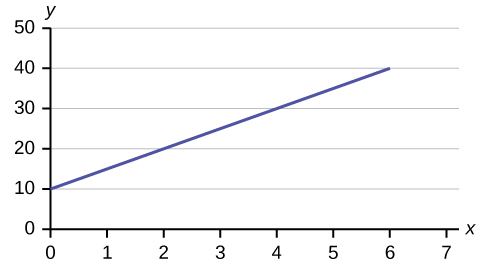
Use the following information to answer the next two exercises. A credit card company charges 💲10 when a payment is late, and 💲5 a day each day the payment remains unpaid.
Find the equation that expresses the total fee in terms of the number of days the payment is late.
Graph the equation from [link].
Solution
Is the equation y = 10 + 5x – 3x2 linear? Why or why not?
Which of the following equations are linear?
a. y = 6x + 8
b. y + 7 = 3x
c. y – x = 8x2
d. 4y = 8
Solution
y = 6x + 8, 4y = 8, and y + 7 = 3x are all linear equations.
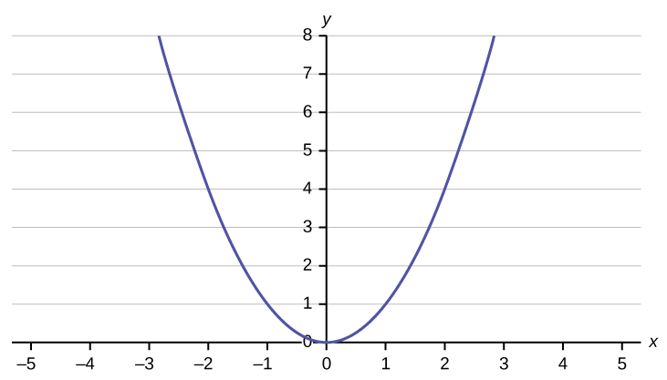
Does the graph show a linear equation? Why or why not?
[link] contains real data for the first two decades of AIDS reporting.
| Year | # AIDS cases diagnosed | # AIDS deaths |
| Pre-1981 | 91 | 29 |
| 1981 | 319 | 121 |
| 1982 | 1,170 | 453 |
| 1983 | 3,076 | 1,482 |
| 1984 | 6,240 | 3,466 |
| 1985 | 11,776 | 6,878 |
| 1986 | 19,032 | 11,987 |
| 1987 | 28,564 | 16,162 |
| 1988 | 35,447 | 20,868 |
| 1989 | 42,674 | 27,591 |
| 1990 | 48,634 | 31,335 |
| 1991 | 59,660 | 36,560 |
| 1992 | 78,530 | 41,055 |
| 1993 | 78,834 | 44,730 |
| 1994 | 71,874 | 49,095 |
| 1995 | 68,505 | 49,456 |
| 1996 | 59,347 | 38,510 |
| 1997 | 47,149 | 20,736 |
| 1998 | 38,393 | 19,005 |
| 1999 | 25,174 | 18,454 |
| 2000 | 25,522 | 17,347 |
| 2001 | 25,643 | 17,402 |
| 2002 | 26,464 | 16,371 |
| Total | 802,118 | 489,093 |
Use the columns “year” and “# AIDS cases diagnosed. Why is “year” the independent variable and “# AIDS cases diagnosed.” the dependent variable (instead of the reverse)?
Solution
The number of AIDS cases depends on the year. Therefore, year becomes the independent variable and the number of AIDS cases is the dependent variable.
Use the following information to answer the next two exercises. A specialty cleaning company charges an equipment fee and an hourly labor fee. A linear equation that expresses the total amount of the fee the company charges for each session is y = 50 + 100x.
What are the independent and dependent variables?
What is the y-intercept and what is the slope? Interpret them using complete sentences.
Solution
The y-intercept is 50 (a = 50). At the start of the cleaning, the company charges a one-time fee of 💲50 (this is when x = 0). The slope is 100 (b = 100). For each session, the company charges 💲100 for each hour they clean.
Use the following information to answer the next three questions. Due to erosion, a river shoreline is losing several thousand pounds of soil each year. A linear equation that expresses the total amount of soil lost per year is y = 12,000x.
What are the independent and dependent variables?
How many pounds of soil does the shoreline lose in a year?
Solution
12,000 pounds of soil
What is the y-intercept? Interpret its meaning.
Use the following information to answer the next two exercises. The price of a single issue of stock can fluctuate throughout the day. A linear equation that represents the price of stock for Shipment Express is y = 15 – 1.5x where x is the number of hours passed in an eight-hour day of trading.
What are the slope and y-intercept? Interpret their meaning.
Solution
The slope is –1.5 (b = –1.5). This means the stock is losing value at a rate of 💲1.50 per hour. The y-intercept is 💲15 (a = 15). This means the price of stock before the trading day was 💲15.
If you owned this stock, would you want a positive or negative slope? Why?
Chapter Review from 10.2
Scatter plots are particularly helpful graphs when we want to see if there is a linear relationship among data points. They indicate both the direction of the relationship between the x variables and the y variables, and the strength of the relationship. We calculate the strength of the relationship between an independent variable and a dependent variable using linear regression.
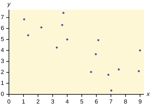
Does the scatter plot appear linear? Strong or weak? Positive or negative?
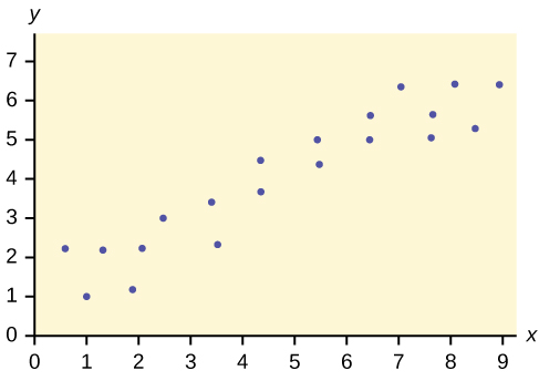
Solution
The data appear to be linear with a strong, positive correlation.
Does the scatter plot appear linear? Strong or weak? Positive or negative?
Does the scatter plot appear linear? Strong or weak? Positive or negative?
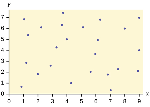
Solution
The data appear to have no correlation.
Chapter Review from 10.3
A regression line, or a line of best fit, can be drawn on a scatter plot and used to predict outcomes for the x and y variables in a given data set or sample data. There are several ways to find a regression line, but usually the least-squares regression line is used because it creates a uniform line. Residuals, also called “errors,” measure the distance from the actual value of y and the estimated value of y. The Sum of Squared Errors, when set to its minimum, calculates the points on the line of best fit. Regression lines can be used to predict values within the given set of data, but should not be used to make predictions for values outside the set of data.
The correlation coefficient r measures the strength of the linear association between x and y. The variable r has to be between –1 and +1. When r is positive, the x and y will tend to increase and decrease together. When r is negative, x will increase and y will decrease, or the opposite, x will decrease and y will increase. The coefficient of determination r2, is equal to the square of the correlation coefficient. When expressed as a percent, r2 represents the percent of variation in the dependent variable y that can be explained by variation in the independent variable x using the regression line.
Use the following information to answer the next five exercises. A random sample of ten professional athletes produced the following data where x is the number of endorsements the player has and y is the amount of money made (in millions of dollars).
| x | y | x | y |
|---|---|---|---|
| 0 | 2 | 5 | 12 |
| 3 | 8 | 4 | 9 |
| 2 | 7 | 3 | 9 |
| 1 | 3 | 0 | 3 |
| 5 | 13 | 4 | 10 |
Draw a scatter plot of the data.
Use regression to find the equation for the line of best fit.
Solution
ŷ = 2.23 + 1.99x
Draw the line of best fit on the scatter plot.
What is the slope of the line of best fit? What does it represent?
Solution
The slope is 1.99 (b = 1.99). It means that for every endorsement deal a professional player gets, he gets an average of another 💲1.99 million in pay each year.
What is the y-intercept of the line of best fit? What does it represent?
What does an r value of zero mean?
Solution
It means that there is no correlation between the data sets.
When n = 2 and r = 1, are the data significant? Explain.
When n = 100 and r = -0.89, is there a significant correlation? Explain.
Solution
Yes, there are enough data points and the value of r is strong enough to show that there is a strong negative correlation between the data sets.
Chapter Review from 10.5
After determining the presence of a strong correlation coefficient and calculating the line of best fit, you can use the least squares regression line to make predictions about your data.
Use the following information to answer the next two exercises. An electronics retailer used regression to find a simple model to predict sales growth in the first quarter of the new year (January through March). The model is good for 90 days, where x is the day. The model can be written as follows:
ŷ = 101.32 + 2.48x where ŷ is in thousands of dollars.
What would you predict the sales to be on day 60?
Solution
💲250,120
What would you predict the sales to be on day 90?
Use the following information to answer the next three exercises. A landscaping company is hired to mow the grass for several large properties. The total area of the properties combined is 1,345 acres. The rate at which one person can mow is as follows:
ŷ = 1350 – 1.2x where x is the number of hours and ŷ represents the number of acres left to mow.
How many acres will be left to mow after 20 hours of work?
Solution
1,326 acres
How many acres will be left to mow after 100 hours of work?
How many hours will it take to mow all of the lawns? (When is ŷ = 0?)
Solution
1,125 hours, or when x = 1,125
[link] contains real data for the first two decades of AIDS reporting.
| Year | # AIDS cases diagnosed | # AIDS deaths |
| Pre-1981 | 91 | 29 |
| 1981 | 319 | 121 |
| 1982 | 1,170 | 453 |
| 1983 | 3,076 | 1,482 |
| 1984 | 6,240 | 3,466 |
| 1985 | 11,776 | 6,878 |
| 1986 | 19,032 | 11,987 |
| 1987 | 28,564 | 16,162 |
| 1988 | 35,447 | 20,868 |
| 1989 | 42,674 | 27,591 |
| 1990 | 48,634 | 31,335 |
| 1991 | 59,660 | 36,560 |
| 1992 | 78,530 | 41,055 |
| 1993 | 78,834 | 44,730 |
| 1994 | 71,874 | 49,095 |
| 1995 | 68,505 | 49,456 |
| 1996 | 59,347 | 38,510 |
| 1997 | 47,149 | 20,736 |
| 1998 | 38,393 | 19,005 |
| 1999 | 25,174 | 18,454 |
| 2000 | 25,522 | 17,347 |
| 2001 | 25,643 | 17,402 |
| 2002 | 26,464 | 16,371 |
| Total | 802,118 | 489,093 |
Graph “year” versus “# AIDS cases diagnosed” (plot the scatter plot). Do not include pre-1981 data.
Perform linear regression. What is the linear equation? Round to the nearest whole number.
Solution
Check student’s solution.
Write the equations:
Solve.
Solution
Does the line seem to fit the data? Why or why not?
What does the correlation imply about the relationship between time (years) and the number of diagnosed AIDS cases reported in the U.S.?
Solution
Also, the correlation r = 0.4526. If r is compared to the value in the 95% Critical Values of the Sample Correlation Coefficient Table, because r > 0.423, r is significant, and you would think that the line could be used for prediction. But the scatter plot indicates otherwise.
<!– From 12.4 Move to 12.8 –>
Plot the two given points on the following graph. Then, connect the two points to form the regression line.
Obtain the graph on your calculator or computer.
<!– From 12.5 MOVE to 12.8 –>
Write the equation: ŷ= ____________
Solution
[latex]\stackrel{^}{y}[/latex] = 3,448,225 + 1750x
Hand draw a smooth curve on the graph that shows the flow of the data.
<!– From 12.6 Move to 12.8 –>
Does the line seem to fit the data? Why or why not?
Solution
There was an increase in AIDS cases diagnosed until 1993. From 1993 through 2002, the number of AIDS cases diagnosed declined each year. It is not appropriate to use a linear regression line to fit to the data.
Do you think a linear fit is best? Why or why not?
What does the correlation imply about the relationship between time (years) and the number of diagnosed AIDS cases reported in the U.S.?
Solution
Since there is no linear association between year and # of AIDS cases diagnosed, it is not appropriate to calculate a linear correlation coefficient. When there is a linear association and it is appropriate to calculate a correlation, we cannot say that one variable “causes” the other variable.
<!– From 12.7 MOVE to 12.8 –>
Graph “year” vs. “# AIDS cases diagnosed.” Do not include pre-1981. Label both axes with words. Scale both axes.
Enter your data into your calculator or computer. The pre-1981 data should not be included. Why is that so?
Write the linear equation, rounding to four decimal places:
Solution
We don’t know if the pre-1981 data was collected from a single year. So we don’t have an accurate x value for this figure.
Regression equation: ŷ (#AIDS Cases) = –3,448,225 + 1749.777 (year)
| Coefficients | |
|---|---|
| Intercept | –3,448,225 |
| X Variable 1 | 1,749.777 |
Calculate the following:
- a = _____
- b = _____
- correlation = _____
- n = _____
Chapter Review from 10.6
To determine if a point is an outlier, do one of the following:
Input the following equations into the TI 83, 83+,84, 84+:
[latex]\begin{array}{l}{y}_{1}=a+bx\hfill \\ {y}_{2}=\left(2s\right)a+bx\hfill \\ {y}_{3}=-\left(2s\right)a+bx\hfill \end{array}[/latex] where s is the standard deviation of the residuals
If any point is above y2or below y3 then the point is considered to be an outlier.
Use the following information to answer the next four exercises. The scatter plot shows the relationship between hours spent studying and exam scores. The line shown is the calculated line of best fit. The correlation coefficient is 0.69.

Do there appear to be any outliers?
Solution
Yes, there appears to be an outlier at (6, 58).
A point is removed, and the line of best fit is recalculated. The new correlation coefficient is 0.98. Does the point appear to have been an outlier? Why?
What effect did the potential outlier have on the line of best fit?
Solution
The potential outlier flattened the slope of the line of best fit because it was below the data set. It made the line of best fit less accurate as a predictor for the data.
Are you more or less confident in the predictive ability of the new line of best fit?
The Sum of Squared Errors for a data set of 18 numbers is 49. What is the standard deviation?
Solution
s = 1.75
The Standard Deviation for the Sum of Squared Errors for a data set is 9.8. What is the cutoff for the vertical distance that a point can be from the line of best fit to be considered an outlier?
