Chapter 11: The Chi-Square Distribution
11.2 Goodness-of-Fit Test
Learning Objectives
By the end of this section, the student should be able to:
- calculate and interpret the Chi-Square Goodness-of-Fit test
In this type of hypothesis test, you determine whether the data “fit” a particular distribution or not. For example, you may suspect your unknown data fit a binomial distribution. You use a chi-square test (meaning the distribution for the hypothesis test is chi-square) to determine if there is a fit or not. The null and the alternative hypotheses for this test may be written in sentences or may be stated as equations or inequalities.
The test statistic for a goodness-of-fit test is:
where:
- O = observed values (data)
- E = expected values (from theory)
- k = the number of different data cells or categories
The observed values are the data values and the expected values are the values you would expect to get if the null hypothesis were true. There are n terms of the form [latex]\frac{{\left(O-E\right)}^{2}}{E}[/latex].
The number of degrees of freedom is df = (number of categories – 1).
The goodness-of-fit test is almost always right-tailed. If the observed values and the corresponding expected values are not close to each other, then the test statistic can get very large and will be way out in the right tail of the chi-square curve.
Note
The expected value for each cell needs to be at least five in order for you to use this test.
Example
Absenteeism of college students from math classes is a major concern to math instructors because missing class appears to increase the drop rate. Suppose that a study was done to determine if the actual student absenteeism rate follows faculty perception. The faculty expected that a group of 100 students would miss class according to [link].
| Number of absences per term | Expected number of students |
|---|---|
| 0–2 | 50 |
| 3–5 | 30 |
| 6–8 | 12 |
| 9–11 | 6 |
| 12+ | 2 |
A random survey across all mathematics courses was then done to determine the actual number (observed) of absences in a course. The chart in [link] displays the results of that survey.
| Number of absences per term | Actual number of students |
|---|---|
| 0–2 | 35 |
| 3–5 | 40 |
| 6–8 | 20 |
| 9–11 | 1 |
| 12+ | 4 |
Determine the null and alternative hypotheses needed to conduct a goodness-of-fit test.
H0: Student absenteeism fits faculty perception.
The alternative hypothesis is the opposite of the null hypothesis.
Ha: Student absenteeism does not fit faculty perception.
a. Can you use the information as it appears in the charts to conduct the goodness-of-fit test?
Solution
a. No. Notice that the expected number of absences for the “12+” entry is less than five (it is two). Combine that group with the “9–11” group to create new tables where the number of students for each entry are at least five. The new results are in [link] and [link].
| Number of absences per term | Expected number of students |
|---|---|
| 0–2 | 50 |
| 3–5 | 30 |
| 6–8 | 12 |
| 9+ | 8 |
| Number of absences per term | Actual number of students |
|---|---|
| 0–2 | 35 |
| 3–5 | 40 |
| 6–8 | 20 |
| 9+ | 5 |
b. What is the number of degrees of freedom (df)?
Solution
b. There are four “cells” or categories in each of the new tables.
df = number of cells – 1 = 4 – 1 = 3
Your Turn!
A factory manager needs to understand how many products are defective versus how many are produced. The number of expected defects is listed in [link].
| Number produced | Number defective |
|---|---|
| 0–100 | 5 |
| 101–200 | 6 |
| 201–300 | 7 |
| 301–400 | 8 |
| 401–500 | 10 |
A random sample was taken to determine the actual number of defects. [link] shows the results of the survey.
| Number produced | Number defective |
|---|---|
| 0–100 | 5 |
| 101–200 | 7 |
| 201–300 | 8 |
| 301–400 | 9 |
| 401–500 | 11 |
State the null and alternative hypotheses needed to conduct a goodness-of-fit test, and state the degrees of freedom.
Solution
H0:The number of defaults fits expectations.
Ha:The number of defaults does not fit expectations.
df = 4
Example
Employers want to know which days of the week employees are absent in a five-day work week. Most employers would like to believe that employees are absent equally during the week. Suppose a random sample of 60 managers were asked on which day of the week they had the highest number of employee absences. The results were distributed as in [link]. For the population of employees, do the days for the highest number of absences occur with equal frequencies during a five-day work week? Test at a 5% significance level.
| Monday | Tuesday | Wednesday | Thursday | Friday | |
|---|---|---|---|---|---|
| Number of Absences | 15 | 12 | 9 | 9 | 15 |
Solution
The null and alternative hypotheses are:
- H0: The absent days occur with equal frequencies, that is, they fit a uniform distribution.
- Ha: The absent days occur with unequal frequencies, that is, they do not fit a uniform distribution.
If the absent days occur with equal frequencies, then, out of 60 absent days (the total in the sample: 15 + 12 + 9 + 9 + 15 = 60), there would be 12 absences on Monday, 12 on Tuesday, 12 on Wednesday, 12 on Thursday, and 12 on Friday. These numbers are the expected (E) values. The values in the table are the observed (O) values or data.
This time, calculate the χ2 test statistic by hand. Make a chart with the following headings and fill in the columns:
- Expected (E) values (12, 12, 12, 12, 12)
- Observed (O) values (15, 12, 9, 9, 15)
- (O – E)
- (O – E)2
- [latex]\frac{{\left(O\text{ – }E\right)}^{2}}{E}[/latex]
Now add (sum) the last column. The sum is three. This is the χ2 test statistic.
To find the p-value, calculate P(χ2 > 3). This test is right-tailed. (Use a computer or calculator to find the p-value. You should get p-value = 0.5578.)
The dfs are the number of cells – 1 = 5 – 1 = 4
Press 2nd DISTR. Arrow down to χ2cdf. Press ENTER. Enter (3,10^99,4). Rounded to four decimal places, you should see 0.5578, which is the p-value.
Next, complete a graph like the following one with the proper labeling and shading. (You should shade the right tail.)
The decision is not to reject the null hypothesis.
Conclusion: At a 5% level of significance, from the sample data, there is not sufficient evidence to conclude that the absent days do not occur with equal frequencies.
TI-83+ and some TI-84 calculators do not have a special program for the test statistic for the goodness-of-fit test. The next example [link] has the calculator instructions. The newer TI-84 calculators have in STAT TESTS the test Chi2 GOF. To run the test, put the observed values (the data) into a first list and the expected values (the values you expect if the null hypothesis is true) into a second list. Press STAT TESTS and Chi2 GOF. Enter the list names for the Observed list and the Expected list. Enter the degrees of freedom and press calculate or draw. Make sure you clear any lists before you start. To Clear Lists in the calculators: Go into STAT EDIT and arrow up to the list name area of the particular list. Press CLEAR and then arrow down. The list will be cleared. Alternatively, you can press STAT and press 4 (for ClrList). Enter the list name and press ENTER.
Your Turn!
Teachers want to know which night each week their students are doing most of their homework. Most teachers think that students do homework equally throughout the week. Suppose a random sample of 49 students were asked on which night of the week they did the most homework. The results were distributed as in [link].
| Sunday | Monday | Tuesday | Wednesday | Thursday | Friday | Saturday | |
|---|---|---|---|---|---|---|---|
| Number of Students | 11 | 8 | 10 | 7 | 10 | 5 | 5 |
From the population of students, do the nights for the highest number of students doing the majority of their homework occur with equal frequencies during a week? What type of hypothesis test should you use?
Solution
df = 6
p-value = 0.6093
We decline to reject the null hypothesis. There is not enough evidence to support that students do not do the majority of their homework equally throughout the week.
Example
One study indicates that the number of televisions that American families have is distributed (this is the given distribution for the American population) as in [link].
| Number of Televisions | Percent |
|---|---|
| 0 | 10 |
| 1 | 16 |
| 2 | 55 |
| 3 | 11 |
| 4+ | 8 |
The table contains expected (E) percentages.
A random sample of 600 families in the far western United States resulted in the data in [link].
| Number of Televisions | Frequency |
|---|---|
| Total = 600 | |
| 0 | 66 |
| 1 | 119 |
| 2 | 340 |
| 3 | 60 |
| 4+ | 15 |
The table contains observed (O) frequency values.
At the 1% significance level, does it appear that the distribution “number of televisions” of far western United States families is different from the distribution for the American population as a whole?
Solution
This problem asks you to test whether the far western United States families distribution fits the distribution of the American families. This test is always right-tailed.
The first table contains expected percentages. To get expected (E) frequencies, multiply the percentage by 600. The expected frequencies are shown in [link].
| Number of Televisions | Percent | Expected Frequency |
|---|---|---|
| 0 | 10 | (0.10)(600) = 60 |
| 1 | 16 | (0.16)(600) = 96 |
| 2 | 55 | (0.55)(600) = 330 |
| 3 | 11 | (0.11)(600) = 66 |
| over 3 | 8 | (0.08)(600) = 48 |
Therefore, the expected frequencies are 60, 96, 330, 66, and 48. In the TI calculators, you can let the calculator do the math. For example, instead of 60, enter 0.10*600.
H0: The “number of televisions” distribution of far western United States families is the same as the “number of televisions” distribution of the American population.
Ha: The “number of televisions” distribution of far western United States families is different from the “number of televisions” distribution of the American population.
Distribution for the test: [latex]{\chi }_{4}^{2}[/latex] where df = (the number of cells) – 1 = 5 – 1 = 4.
df ≠ 600 – 1
Calculate the test statistic:χ2 = 29.65
Graph:
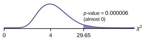
Probability statement: p-value = P(χ2 > 29.65) = 0.000006
Compare α and the p-value:
So, α > p-value.
Make a decision: Since α > p-value, reject Ho.
This means you reject the belief that the distribution for the far western states is the same as that of the American population as a whole.
Conclusion: At the 1% significance level, from the data, there is sufficient evidence to conclude that the “number of televisions” distribution for the far western United States is different from the “number of televisions” distribution for the American population as a whole.
Press STAT and ENTER. Make sure to clear lists L1, L2, and L3 if they have data in them (see the note at the end of [link]). Into L1, put the observed frequencies 66, 119, 349, 60, 15. Into L2, put the expected frequencies .10*600, .16*600, .55*600, .11*600, .08*600. Arrow over to list L3 and up to the name area “L3”. Enter (L1-L2)^2/L2 and ENTER. Press 2nd QUIT. Press 2nd LIST and arrow over to MATH. Press 5. You should see “sum” (Enter L3). Rounded to 2 decimal places, you should see 29.65. Press 2nd DISTR. Press 7 or Arrow down to 7:χ2cdf and press ENTER. Enter (29.65,1E99,4). Rounded to four places, you should see 5.77E-6 = .000006 (rounded to six decimal places), which is the p-value.
The newer TI-84 calculators have in STAT TESTS the test Chi2 GOF. To run the test, put the observed values (the data) into a first list and the expected values (the values you expect if the null hypothesis is true) into a second list. Press STAT TESTS and Chi2 GOF. Enter the list names for the Observed list and the Expected list. Enter the degrees of freedom and press calculate or draw. Make sure you clear any lists before you start.
Your Turn!
The expected percentage of the number of pets students have in their homes is distributed (this is the given distribution for the student population of the United States) as in [link].
| Number of Pets | Percent |
|---|---|
| 0 | 18 |
| 1 | 25 |
| 2 | 30 |
| 3 | 18 |
| 4+ | 9 |
A random sample of 1,000 students from the Eastern United States resulted in the data in [link].
| Number of Pets | Frequency |
|---|---|
| 0 | 210 |
| 1 | 240 |
| 2 | 320 |
| 3 | 140 |
| 4+ | 90 |
At the 1% significance level, does it appear that the distribution “number of pets” of students in the Eastern United States is different from the distribution for the United States student population as a whole? What is the p-value?
Solution
p-value = 0.0036
We reject the null hypothesis that the distributions are the same. There is sufficient evidence to conclude that the distribution “number of pets” of students in the Eastern United States is different from the distribution for the United States student population as a whole.
Example
Suppose you flip two coins 100 times. The results are 20 HH, 27 HT, 30 TH, and 23 TT. Are the coins fair? Test at a 5% significance level.
Solution
This problem can be set up as a goodness-of-fit problem. The sample space for flipping two fair coins is {HH, HT, TH, TT}. Out of 100 flips, you would expect 25 HH, 25 HT, 25 TH, and 25 TT. This is the expected distribution. The question, “Are the coins fair?” is the same as saying, “Does the distribution of the coins (20 HH, 27 HT, 30 TH, 23 TT) fit the expected distribution?”
Random Variable: Let X = the number of heads in one flip of the two coins. X takes on the values 0, 1, 2. (There are 0, 1, or 2 heads in the flip of two coins.) Therefore, the number of cells is three. Since X = the number of heads, the observed frequencies are 20 (for two heads), 57 (for one head), and 23 (for zero heads or both tails). The expected frequencies are 25 (for two heads), 50 (for one head), and 25 (for zero heads or both tails). This test is right-tailed.
H0: The coins are fair.
Ha: The coins are not fair.
Distribution for the test:[latex]{\chi }_{2}^{2}[/latex]
where
df = 3 – 1 = 2.
Calculate the test statistic:χ2 = 2.14
Graph:
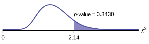
Probability statement:p-value = P(χ2 > 2.14) = 0.3430
Compare α and the p-value:
α < p-value.
Make a decision: Since α < p-value, do not reject H0.
Conclusion: There is insufficient evidence to conclude that the coins are not fair.
Press STAT and ENTER. Make sure you
clear lists L1, L2, and L3 if they have data in them. Into L1, put the observed
frequencies 20, 57, 23. Into L2, put the expected frequencies 25, 50, 25. Arrow
over to list L3 and up to the name area “L3”. Enter (L1-L2)^2/L2 and
ENTER. Press 2nd QUIT. Press 2nd LIST and arrow over to MATH. Press
5. You should see “sum”. Enter L3. Rounded to two decimal places, you
should see 2.14. Press 2nd DISTR. Arrow down to 7:χ2cdf (or press 7). Press
ENTER. Enter 2.14,1E99,2). Rounded to four places, you should see .3430, which
is the p-value.
The newer TI-84 calculators have in STAT TESTS the test Chi2 GOF. To run the test, put the observed values (the data) into a first list and the expected values (the values you expect if the null hypothesis is true) into a second list. Press STAT TESTS and Chi2 GOF. Enter the list names for the Observed list and the Expected list. Enter the degrees of freedom and press calculate or draw. Make
sure you clear any lists before you start.
Your Turn!
Students in a social studies class hypothesize that the literacy rates across the world for every region are 82%. [link] shows the actual literacy rates across the world broken down by region. What are the test statistics and the degrees of freedom?
| MDG Region | Adult Literacy Rate (%) |
|---|---|
| Developed Regions | 99.0 |
| Commonwealth of Independent States | 99.5 |
| Northern Africa | 67.3 |
| Sub-Saharan Africa | 62.5 |
| Latin America and the Caribbean | 91.0 |
| Eastern Asia | 93.8 |
| Southern Asia | 61.9 |
| South-Eastern Asia | 91.9 |
| Western Asia | 84.5 |
| Oceania | 66.4 |
Solution
degrees of freedom = 9
chi2 test statistic = 26.38
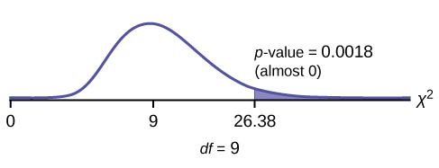
Press STAT and ENTER. Make sure you clear lists L1, L2, and L3 if they have data in them. Into L1, put the observed frequencies 99, 99.5, 67.3, 62.5, 91, 93.8, 61.9, 91.9, 84.5, 66.4. Into L2, put the expected frequencies 82, 82, 82, 82, 82, 82, 82, 82, 82, 82. Arrow over to list L3 and up to the name area "L3". Enter (L1-L2)^2/L2 and ENTER. Press 2nd QUIT. Press 2nd LIST and arrow over to MATH. Press 5. You should see "sum". Enter L3. Rounded to two decimal places, you should see 26.38. Press 2nd DISTR. Arrow down to 7:χ2cdf (or press 7). Press ENTER. Enter 26.38,1E99,9). Rounded to four places, you should see .0018, which is the p-value.
The newer TI-84 calculators have in STAT TESTS the test Chi2 GOF. To run the test, put the observed values (the data) into a first list and the expected values (the values you expect if the null hypothesis is true) into a second list. Press STAT TESTS and Chi2 GOF. Enter the list names for the Observed list and the Expected list. Enter the degrees of freedom and press calculate or draw. Make sure you clear any lists before you start.
References
Data from the U.S. Census Bureau
Data from the College Board. Available online at http://www.collegeboard.com.
Data from the U.S. Census Bureau, Current Population Reports.
Ma, Y., E.R. Bertone, E.J. Stanek III, G.W. Reed, J.R. Hebert, N.L. Cohen, P.A. Merriam, I. S. Ockene, “Association between Eating Patterns and Obesity in a Free-living US Adult Population.” American Journal of Epidemiology volume 158, no. 1, pages 85-92.
Ogden, Cynthia L., Margaret D. Carroll, Brian K. Kit, Katherine M. Flegal, “Prevalence of Obesity in the United States, 2009–2010.” NCHS Data Brief no. 82, January 2012. Available online at http://www.cdc.gov/nchs/data/databriefs/db82.pdf (accessed May 24, 2013).
Stevens, Barbara J., “Multi-family and Commercial Solid Waste and Recycling Survey.” Arlington Count, VA. Available online at http://www.arlingtonva.us/departments/EnvironmentalServices/SW/file84429.pdf (accessed May 24,2013).
Use the following information to answer the next nine exercises: The following data are real. The cumulative number of AIDS cases reported for Santa Clara County is broken down by ethnicity as in [link].
