Chapter 9: Hypothesis Testing with Two Samples
9.4 Matched or Paired Samples
Learning Objectives
By the end of this section, the student should be able to
- Conduct and interpret hypothesis tests for matched or paired samples.
Hypothesis Tests for Matched or Paired Samples
When using a hypothesis test for matched or paired samples, the following characteristics should be present:
- Simple random sampling is used.
- Sample sizes are often small.
- Two measurements (samples) are drawn from the same pair of individuals or objects.
- Differences are calculated from the matched or paired samples.
- The differences form the sample that is used for the hypothesis test.
- Either the matched pairs have differences that come from a population that is normal or the number of differences is sufficiently large so that distribution of the sample mean of differences is approximately normal.
In a hypothesis test for matched or paired samples, subjects are matched in pairs and differences are calculated. The differences are the data. The population mean for the differences, [latex]\mu_d[/latex], is then tested using a Student’s t-test for a single population mean with [latex]n – 1[/latex] degrees of freedom, where [latex]n[/latex] is the number of differences.
The test statistic (t-score) is: [latex]t=\frac{{\overline{x}}_{d}-{\mu }_{d}}{\left(\frac{{s}_{d}}{\sqrt{n}}\right)}[/latex]
Example
A study was conducted to investigate the effectiveness of hypnotism in reducing pain. Results for randomly selected subjects are shown in the table below. A lower score indicates less pain. The “before” value is matched to an “after” value and the differences are calculated. The differences have a normal distribution. Are the sensory measurements, on average, lower after hypnotism? Test at a 5% significance level.
| Subject: | A | B | C | D | E | F | G | H |
|---|---|---|---|---|---|---|---|---|
| Before | 6.6 | 6.5 | 9.0 | 10.3 | 11.3 | 8.1 | 6.3 | 11.6 |
| After | 6.8 | 2.4 | 7.4 | 8.5 | 8.1 | 6.1 | 3.4 | 2.0 |
Solution
Corresponding “before” and “after” values form matched pairs. (Calculate “after” – “before.”)
| After Data | Before Data | Difference |
|---|---|---|
| 6.8 | 6.6 | 0.2 |
| 2.4 | 6.5 | -4.1 |
| 7.4 | 9 | -1.6 |
| 8.5 | 10.3 | -1.8 |
| 8.1 | 11.3 | -3.2 |
| 6.1 | 8.1 | -2 |
| 3.4 | 6.3 | -2.9 |
| 2 | 11.6 | -9.6 |
The data for the test are the differences: {0.2, –4.1, –1.6, –1.8, –3.2, –2, –2.9, –9.6}
The sample mean and sample standard deviation of the differences are [latex]\overline{{x}_{d}}=–3.13[/latex] and [latex]{s}_{d}=2.91[/latex]
Verify these values.
Let [latex]{\mu }_{d}[/latex] be the population mean for the differences. We use the subscript [latex]d[/latex] to denote “differences.”
Random variable:[latex]{\overline{X}}_{d}[/latex] = the mean difference of the sensory measurements
[latex]H_0: \mu_d \ge 0[/latex]
The null hypothesis is zero or positive, meaning that there is the same or more pain felt after hypnotism. That means the subject shows no improvement. μd is the population mean of the differences.
[latex]H_a: \mu_d \lt 0[/latex]
The alternative hypothesis is negative, meaning there is less pain felt after hypnotism. That means the subject shows improvement. The score should be lower after hypnotism, so the difference ought to be negative to indicate improvement.
Distribution for the test: The distribution is a Student’s t with [latex]df = n – 1 = 8 – 1 = 7[/latex]. Use [latex]t_7[/latex]. (Notice that the test is for a single population mean.)
Calculate the p-value using the Student’s t-distribution: [latex]\text{p-value} = 0.0095[/latex]
Graph:
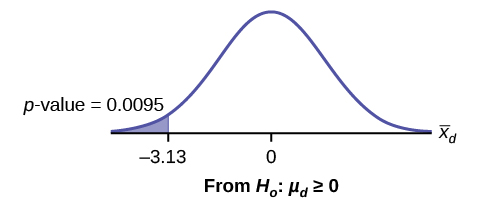
[latex]{\overline{X}}_{d}[/latex] is the random variable for the differences.
The sample mean and sample standard deviation of the differences are:
[latex]{\overline{x}}_{d} = -3.13[/latex]
[latex]{\overline{s}}_{d} = 2.9[/latex]
Compare α and the p-value: [latex]\alpha = 0.05[/latex] and [latex]\text{p-value} = 0.0095[/latex], so [latex]\alpha > \text{p-value}[/latex].
Make a decision: Since [latex]\alpha > \text{p-value}[/latex], reject [latex]H_0[/latex]. This means that [latex]\mu_d \lt 0[/latex] and there is improvement.
Conclusion: At a 5% level of significance, from the sample data, there is sufficient evidence to conclude that the sensory measurements, on average, are lower after hypnotism. Hypnotism appears to be effective in reducing pain.
Note
For the TI-83+ and TI-84 calculators, you can either calculate the differences ahead of time (after – before) and put the differences into a list or you can put the after data into a first list and the before data into a second list. Then go to a third list and arrow up to the name. Enter 1st list name – 2nd list name. The calculator will do the subtraction, and you will have the differences in the third list.
Use your list of differences as the data. Press STAT and arrow over to TESTS. Press 2:T-Test. Arrow over to Data and press ENTER. Arrow down and enter 0 for [latex]{\mu }_{0}[/latex], the name of the list where you put the data, and 1 for Freq:. Arrow down to μ: and arrow over to < [latex]{\mu }_{0}[/latex]. Press ENTER. Arrow down to Calculate and press ENTER. The p-value is 0.0094, and the test statistic is -3.04. Do these instructions again except, arrow to Draw (instead of Calculate). Press ENTER.
Your Turn!
A study was conducted to investigate how effective a new diet was in lowering cholesterol. Results for the randomly selected subjects are shown in the table. The differences have a normal distribution. Are the subjects’ cholesterol levels lower on average after the diet? Test at the 5% level.
| Subject | A | B | C | D | E | F | G | H | I |
| Before | 209 | 210 | 205 | 198 | 216 | 217 | 238 | 240 | 222 |
| After | 199 | 207 | 189 | 209 | 217 | 202 | 211 | 223 | 201 |
Solution
The p-value is 0.0130, so we can reject the null hypothesis. There is enough evidence to suggest that the diet lowers cholesterol.
Example
A college football coach was interested in whether the college’s strength development class increased his players’ maximum lift (in pounds) on the bench press exercise. He asked four of his players to participate in a study. The amount of weight they could each lift was recorded before they took the strength development class. After completing the class, the amount of weight they could each lift was again measured. The data are as follows:
| Weight (in pounds) | Player 1 | Player 2 | Player 3 | Player 4 |
|---|---|---|---|---|
| Amount of weight lifted prior to the class | 205 | 241 | 338 | 368 |
| Amount of weight lifted after the class | 295 | 252 | 330 | 360 |
The coach wants to know if the strength development class makes his players stronger, on average.
Record the differences data. Calculate the differences by subtracting the amount of weight lifted prior to the class from the weight lifted after completing the class. The data for the differences are: {90, 11, -8, -8}. Assume the differences have a normal distribution.
Using the differences data, calculate the sample mean and the sample standard deviation.
[latex]{\overline{x}}_{d} = 21.3[/latex], [latex]s_d = 46.7[/latex]
Note: The data given here would indicate that the distribution is actually right-skewed. The difference 90 may be an extreme outlier? It is pulling the sample mean to be 21.3 (positive). The means of the other three data values are actually negative.
Using the difference data, this becomes a test of a single [latex]\underline{\hspace{2cm}}[/latex] (fill in the blank).
Define the random variable:[latex]{\overline{X}}_{d}[/latex] mean difference in the maximum lift per player.
The distribution for the hypothesis test is [latex]t_3[/latex].
[latex]H_0: \mu_d \le 0, H_a: \mu_d > 0[/latex]
Graph:
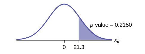
Calculate the p-value: The p-value is 0.2150
Decision: If the level of significance is 5%, the decision is not to reject the null hypothesis, because [latex]\alpha \lt \text{p-value}[/latex].
What is the conclusion?
At a 5% level of significance, from the sample data, there is not sufficient evidence to conclude that the strength development class helped to make the players stronger, on average.
Your Turn!
A new prep class was designed to improve SAT test scores. Five students were selected at random. Their scores on two practice exams were recorded, one before the class and one after. The data recorded in the table below. Are the scores, on average, higher after the class? Test at a 5% level.
| SAT Scores | Student 1 | Student 2 | Student 3 | Student 4 |
|---|---|---|---|---|
| Score before class | 1840 | 1960 | 1920 | 2150 |
| Score after class | 1920 | 2160 | 2200 | 2100 |
Solution
The p-value is 0.0874, so we decline to reject the null hypothesis. The data do not support that the class improves SAT scores significantly.
Example
Seven eighth graders at Kennedy Middle School measured how far they could push the shot-put with their dominant (writing) hand and their weaker (non-writing) hand. They thought that they could push equal distances with either hand. The data were collected and recorded in the table below.
| Distance (in feet) using | Student 1 | Student 2 | Student 3 | Student 4 | Student 5 | Student 6 | Student 7 |
|---|---|---|---|---|---|---|---|
| Dominant Hand | 30 | 26 | 34 | 17 | 19 | 26 | 20 |
| Weaker Hand | 28 | 14 | 27 | 18 | 17 | 26 | 16 |
Conduct a hypothesis test to determine whether the mean difference in distances between the children’s dominant versus weaker hands is significant.
Record the differences data. Calculate the differences by subtracting the distances with the weaker hand from the distances with the dominant hand. The data for the differences are: {2, 12, 7, –1, 2, 0, 4}. The differences have a normal distribution.
Using the differences data, calculate the sample mean and the sample standard deviation. [latex]{\overline{x}}_{d} = 3.71[/latex], [latex]{s}_{d} = 4.5[/latex]
Random variable:[latex]{\overline{X}}_{d}[/latex] = mean difference in the distances between the hands.
Distribution for the hypothesis test:[latex]t_6[/latex]
[latex]H_0: \mu_d = 0[/latex], and [latex]H_a: \mu_d \neq 0[/latex]
Graph:
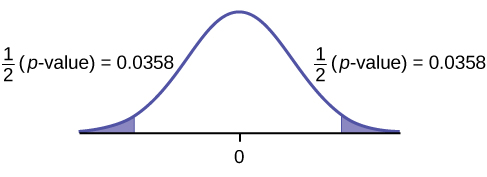
Calculate the p-value: The p-value is 0.0716 (using the data directly).
([latex]\text{test statistic} = 2.18[/latex], [latex]\text{p-value} = 0.0719[/latex] using [latex]\left({\overline{x}}_{d}=3.71, {s}_{d}=4.5\right)[/latex])
Decision: Assume [latex]\alpha = 0.05[/latex]. Since [latex]\alpha \lt \text{p-value}[/latex], Do not reject [latex]H_0[/latex].
Conclusion: At the 5% level of significance, from the sample data, there is not sufficient evidence to conclude that there is a difference in the children’s weaker and dominant hands to push the shot-put.
Your Turn!
Five ball players think they can throw the same distance with their dominant hand (throwing) and off-hand (catching hand). The data were collected and recorded in the table below. Conduct a hypothesis test to determine whether the mean difference in distances between the dominant and off-hand is significant. Test at the 5% level.
| Player 1 | Player 2 | Player 3 | Player 4 | Player 5 | |
|---|---|---|---|---|---|
| Dominant Hand | 120 | 111 | 135 | 140 | 125 |
| Off-hand | 105 | 109 | 98 | 111 | 99 |
Solution
The p-level is 0.0230, so we can reject the null hypothesis. The data show that the players do not throw the same distance with their off-hands as they do with their dominant hands.
Section 9.4 Review
A hypothesis test for matched or paired samples (t-test) has these characteristics:
- Test the differences by subtracting one measurement from the other measurement
- Random Variable: [latex]{\overline{x}}_{d}[/latex] = mean of the differences
- Distribution: Student’s-t distribution with [latex]n – 1[/latex] degrees of freedom
- If the number of differences is small (less than 30), the differences must follow a normal distribution.
- Two samples are drawn from the same set of objects.
- Samples are dependent.
Formula Review
- Test Statistic (t-score):
-
- [latex]t = \frac{{\overline{x}}_{d}-{\mu }_{d}}{\left(\frac{{s}_{d}}{\sqrt{n}}\right)}[/latex]
- [latex]{\overline{x}}_{d}[/latex] is the mean of the sample differences.
- [latex]\mu_d[/latex] is the mean of the population differences.
- [latex]s_d[/latex] is the sample standard deviation of the differences.
- [latex]n[/latex] is the sample size.
Section 9.4 Practice
Use the following information to answer the next five exercises. A study was conducted to test the effectiveness of a software patch in reducing system failures over a six-month period. Results for randomly selected installations are shown in the table below. The “before” value is matched to an “after” value, and the differences are calculated. The differences have a normal distribution. Test at the 1% significance level.
| Installation | A | B | C | D | E | F | G | H |
|---|---|---|---|---|---|---|---|---|
| Before | 3 | 6 | 4 | 2 | 5 | 8 | 2 | 6 |
| After | 1 | 5 | 2 | 0 | 1 | 0 | 2 | 2 |
1. What is the random variable?
Solution
the mean difference of the system failures
2. State the null and alternative hypotheses.
3. What is the p-value?
Solution
0.0067
4. Draw the graph of the p-value.
5. What conclusion can you draw about the software patch?
Solution
With a p-value 0.0067, we can reject the null hypothesis. There is enough evidence to support that the software patch is effective in reducing the number of system failures.
Use the following information to answer the next five exercises. A study was conducted to test the effectiveness of a juggling class. Before the class started, six subjects juggled as many balls as they could at once. After the class, the same six subjects juggled as many balls as they could. The differences in the number of balls are calculated. The differences have a normal distribution. Test at the 1% significance level.
| Subject | A | B | C | D | E | F |
|---|---|---|---|---|---|---|
| Before | 3 | 4 | 3 | 2 | 4 | 5 |
| After | 4 | 5 | 6 | 4 | 5 | 7 |
1. State the null and alternative hypotheses.
2. What is the p-value?
Solution
0.0021
3. What is the sample mean difference?
4. Draw the graph of the p-value.
Solution
5. What conclusion can you draw about the juggling class?
Use the following information to answer the next five exercises. A doctor wants to know if a blood pressure medication is effective. Six subjects have their blood pressures recorded. After twelve weeks on the medication, the same six subjects have their blood pressure recorded again. For this test, only systolic pressure is of concern. Test at the 1% significance level.
| Patient | A | B | C | D | E | F |
|---|---|---|---|---|---|---|
| Before | 161 | 162 | 165 | 162 | 166 | 171 |
| After | 158 | 159 | 166 | 160 | 167 | 169 |
1. State the null and alternative hypotheses.
Solution
[latex]H_0: \mu_d \ge 0[/latex]
[latex]H_a: \mu_d \lt 0[/latex]
2. What is the test statistic?
3. What is the p-value?
Solution
0.0699
4. What is the sample mean difference?
5. What is the conclusion?
Solution
We decline to reject the null hypothesis. There is not sufficient evidence to support that the medication is effective.
For each of the following word problems, use a solution sheet to do the hypothesis test. The solution sheet is found in Chapter 9 Introduction.
Note: If you are using a Student’s t-distribution for the homework problems, including for paired data, you may assume that the underlying population is normally distributed. (When using these tests in a real situation, you must first prove that assumption, however.)
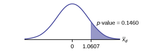
Ten individuals went on a low–fat diet for 12 weeks to lower their cholesterol. The data are recorded in the table below. Do you think that their cholesterol levels were significantly lowered?
| Starting cholesterol level | Ending cholesterol level |
|---|---|
| 140 | 140 |
| 220 | 230 |
| 110 | 120 |
| 240 | 220 |
| 200 | 190 |
| 180 | 150 |
| 190 | 200 |
| 360 | 300 |
| 280 | 300 |
| 260 | 240 |
Solution
p-value = 0.1494
At the 5% significance level, there is insufficient evidence to conclude that the medication lowered cholesterol levels after 12 weeks.
Use the following information to answer the next two exercises. A new AIDS prevention drug was tried on a group of 224 HIV positive patients. Forty-five patients developed AIDS after four years. In a control group of 224 HIV positive patients, 68 developed AIDS after four years. We want to test whether the method of treatment reduces the proportion of patients that develop AIDS after four years or if the proportions of the treated group and the untreated group stay the same.
Let the subscript t = treated patient and ut = untreated patient.
1. The appropriate hypotheses are:
a. [latex]H_0: p_t \lt p_{ut} and H_a: p_t \ge p_{ut}[/latex]
b. [latex]H_0: p_t \le p_{ut} and H_a: p_t > p_{ut}[/latex]
c. [latex]H_0: p_t = p_{ut} and H_a: p_t \neq p_{ut}[/latex]
d. [latex]H_0: p_t = p_{ut} and H_a: p_t \lt p_{ut}[/latex]
2. If the p-value is 0.0062 what is the conclusion (use [latex]\alpha = 0.05[/latex])?
a. The method has no effect.
b. There is sufficient evidence to conclude that the method reduces the proportion of HIV positive patients who develop AIDS after four years.
c. There is sufficient evidence to conclude that the method increases the proportion of HIV positive patients who develop AIDS after four years.
d. There is insufficient evidence to conclude that the method reduces the proportion of HIV positive patients who develop AIDS after four years.
Solution
b
Use the following information to answer the next two exercises. An experiment is conducted to show that blood pressure can be consciously reduced in people trained in a “biofeedback exercise program.” Six subjects were randomly selected and blood pressure measurements were recorded before and after the training. The difference between blood pressures was calculated (after – before) producing the following results: [latex]{\overline{x}}_{d} = -10.2; s_d = 8.4.[/latex] Using the data, test the hypothesis that the blood pressure has decreased after the training.
The distribution for the test is:
a. [latex]t_5[/latex]
b. [latex]t_6[/latex]
c. [latex]N(−10.2, 8.4)[/latex]
d. [latex]N(−10.2, \frac{8.4}{\sqrt{6}})[/latex]
If [latex]\alpha = 0.05[/latex], the p-value and the conclusion are
a. 0.0014; There is sufficient evidence to conclude that the blood pressure decreased after the training.
b. 0.0014; There is sufficient evidence to conclude that the blood pressure increased after the training.
c. 0.0155; There is sufficient evidence to conclude that the blood pressure decreased after the training.
d. 0.0155; There is sufficient evidence to conclude that the blood pressure increased after the training.
Solution
c
A golf instructor is interested in determining if her new technique for improving players’ golf scores is effective. She takes four new students. She records their 18-hole scores before learning the technique and then after having taken her class. She conducts a hypothesis test. The data are as follows.
| Player 1 | Player 2 | Player 3 | Player 4 | |
|---|---|---|---|---|
| Mean score before class | 83 | 78 | 93 | 87 |
| Mean score after class | 80 | 80 | 86 | 86 |
The correct decision is:
a. Reject [latex]H_0[/latex].
b. Do not reject the [latex]H_0[/latex].
A local cancer support group believes that the estimate for new female breast cancer cases in the south is higher in 2013 than in 2012. The group compared the estimates of new female breast cancer cases by southern state in 2012 and in 2013. The results are in the table below.
| Southern States | 2012 | 2013 |
|---|---|---|
| Alabama | 3,450 | 3,720 |
| Arkansas | 2,150 | 2,280 |
| Florida | 15,540 | 15,710 |
| Georgia | 6,970 | 7,310 |
| Kentucky | 3,160 | 3,300 |
| Louisiana | 3,320 | 3,630 |
| Mississippi | 1,990 | 2,080 |
| North Carolina | 7,090 | 7,430 |
| Oklahoma | 2,630 | 2,690 |
| South Carolina | 3,570 | 3,580 |
| Tennessee | 4,680 | 5,070 |
| Texas | 15,050 | 14,980 |
| Virginia | 6,190 | 6,280 |
Solution
Test: two matched pairs or paired samples (t-test)
Random variable: [latex]{\overline{X}}_{d}[/latex]
Distribution: [latex]t_{12}[/latex]
[latex]H_0: \mu_d = 0; H_a: \mu_d > 0[/latex]
The mean of the differences of new female breast cancer cases in the south between 2013 and 2012 is greater than zero. The estimate for new female breast cancer cases in the south is higher in 2013 than in 2012.
Graph: right-tailed
p-value: 0.0004
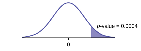
Decision: Reject [latex]H_0[/latex]
Conclusion: At the 5% level of significance, from the sample data, there is sufficient evidence to conclude that there was a higher estimate of new female breast cancer cases in 2013 than in 2012.
A traveler wanted to know if the prices of hotels are different in the ten cities that he visits the most often. The list of the cities with the corresponding hotel prices for his two favorite hotel chains is in the table below. Test at the 1% level of significance.
| Cities | Hyatt Regency prices in dollars | Hilton prices in dollars |
|---|---|---|
| Atlanta | 107 | 169 |
| Boston | 358 | 289 |
| Chicago | 209 | 299 |
| Dallas | 209 | 198 |
| Denver | 167 | 169 |
| Indianapolis | 179 | 214 |
| Los Angeles | 179 | 169 |
| New York City | 625 | 459 |
| Philadelphia | 179 | 159 |
| Washington, DC | 245 | 239 |
A politician asked his staff to determine whether the underemployment rate in the northeast decreased from 2011 to 2012. The results are in the table below.
| Northeastern States | 2011 | 2012 |
|---|---|---|
| Connecticut | 17.3 | 16.4 |
| Delaware | 17.4 | 13.7 |
| Maine | 19.3 | 16.1 |
| Maryland | 16.0 | 15.5 |
| Massachusetts | 17.6 | 18.2 |
| New Hampshire | 15.4 | 13.5 |
| New Jersey | 19.2 | 18.7 |
| New York | 18.5 | 18.7 |
| Ohio | 18.2 | 18.8 |
| Pennsylvania | 16.5 | 16.9 |
| Rhode Island | 20.7 | 22.4 |
| Vermont | 14.7 | 12.3 |
| West Virginia | 15.5 | 17.3 |
Solution
Test: matched or paired samples (t-test)
Difference data: {–0.9, –3.7, –3.2, –0.5, 0.6, –1.9, –0.5, 0.2, 0.6, 0.4, 1.7, –2.4, 1.8}
Random Variable: [latex]{\overline{X}}_{d}[/latex]
Distribution: [latex]H_0: \mu_d = 0; H_a: \mu_d \lt 0[/latex]
The mean of the differences of the rate of underemployment in the northeastern states between 2012 and 2011 is less than zero. The underemployment rate went down from 2011 to 2012.
Graph: left-tailed.
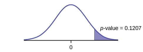
p-value: 0.1207
Decision: Do not reject [latex]H_0[/latex].
Conclusion: At the 5% level of significance, from the sample data, there is not sufficient evidence to conclude that there was a decrease in the underemployment rates of the northeastern states from 2011 to 2012.
