Chapter 6: The Normal Distribution and The Central Limit Theorem
6.3 The Central Limit Theorem for Sample Means (Averages)
Learning Objectives
By the end of this section, the student should be able to:
- Recognize characteristics of the Central Limit Theorem for the Sample Means
- Apply and interpret the Central Limit Theorem for the Sample Means and use it to solve real-world applications.
Applying the law of large numbers here, we could say that if you take larger and larger samples from a population, then the mean [latex]\overline{x}[/latex] of the sample tends to get closer and closer to μ. From the central limit theorem, we know that as n gets larger and larger, the sample means follow a normal distribution. The larger n gets, the smaller the standard deviation gets. (Remember that the standard deviation for [latex]\overline{x}[/latex] is [latex]\frac{\sigma }{\sqrt{n}}[/latex].) This means that the sample mean [latex]\overline{x}[/latex] must be close to the population mean μ. We can say that μ is the value that the sample means approach as n gets larger. The central limit theorem illustrates the law of large numbers.
The size of the sample, n, that is required in order to be “large enough” depends on the original population from which the samples are drawn (the sample size should be at least 30 or the data should come from a normal distribution). If the original population is far from normal, then more observations are needed for the sample means or sums to be normal. Sampling is done with replacement.
The following images look at sampling distributions of the sample mean built from taking 1000 samples of different sample sizes from a normal Population. What pattern do you notice?
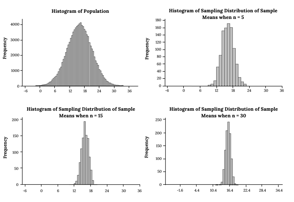
What differences do you notice when sampling from a normal population vs. non-normal?
Example
Suppose:
- eight students roll one fair die ten times
- seven roll two fair dice ten times
- nine roll five fair dice ten times
- 11 roll ten fair dice ten times.
Each time a person rolls more than one die, he or she calculates the sample mean of the faces showing. For example, one person might roll five fair dice and get 2, 2, 3, 4, 6 on one roll.
The mean is [latex]\frac{\text{2 + 2 + 3 + 4 + 6}}{5}[/latex] = 3.4. The 3.4 is one mean when five fair dice are rolled. This same person would roll the five dice nine more times and calculate nine more means for a total of ten means.
As the number of dice rolled increases from one to two to five to ten, the following would happen:
- The mean of the sample means remains approximately the same.
- The spread of the sample means (the standard deviation of the sample means) gets smaller.
- The graph appears steeper and thinner.
We have just demonstrated the idea of central limit theorem (clt) for means, that as you increase the sample size, the sampling distribution of the sample mean tends toward a normal distribution.
To summarize, the central limit theorem for sample means says that if you keep drawing larger and larger samples (such as rolling one, two, five, and finally, ten dice) and calculating their means, the sample means form their own normal distribution (the sampling distribution). The normal distribution has the same mean as the original distribution and a variance that equals the original variance divided by the sample size. Standard deviation is the square root of variance, so the standard deviation of the sampling distribution (a.k.a. standard error) is the standard deviation of the original distribution divided by the square root of n. The variable n is the number of values that are averaged together, not the number of times the experiment is done.
It would be difficult to overstate the importance of the central limit theorem in statistical theory. Knowing that data, even if its distribution is not normal, behaves in a predictable way is a powerful tool. We can simulate this idea using technology.
Suppose X is a random variable with a distribution that may be known or unknown (it can be any distribution). Using a subscript that matches the random variable, suppose:
- μX = the mean of X
- σX = the standard deviation of X
If you draw random samples of size n, then as n increases, the random variable [latex]\overline{X}[/latex] which consists of sample means, tends to be normally distributed and [latex]\overline{X}[/latex] ~ N[latex]\left({\mu }_{x}\text{, }\frac{\sigma x}{\sqrt{n}}\right)[/latex].
The central limit theorem for sample means says that if you keep drawing larger and larger samples (such as rolling one, two, five, and finally, ten dice) and calculating their means, the sample means form their own normal distribution (the sampling distribution). The normal distribution has the same mean as the original distribution and a variance that equals the original variance divided by the sample size. The variable n is the number of values that are averaged together, not the number of times the experiment is done.
To put it more formally, if you draw random samples of size n, the distribution of the random variable [latex]\overline{X}[/latex], which consists of sample means, is called the sampling distribution of the mean. The sampling distribution of the mean approaches a normal distribution as n, the sample size, increases.
The random variable [latex]\overline{X}[/latex] has a different z-score associated with it from that of the random variable X. The mean [latex]\overline{x}[/latex] is the value of [latex]\overline{X}[/latex] in one sample.
μX is the average of both X and [latex]\overline{X}[/latex].
[latex]\sigma \overline{x}\text{ = }\frac{\sigma x}{\sqrt{n}}[/latex] = standard deviation of [latex]\overline{X}[/latex] and is called the standard error of the mean.
Using the CLT
The random variable [latex]\overline{X}[/latex] has a different z-score formula associated with it from that of a single observation. Remember, the mean [latex]\overline{x}[/latex] is the mean of one sample and μX is the average, or center, of both X (The original distribution) and [latex]\overline{X}[/latex].
[latex]z=\frac{\overline{x}-{\mu }_{x}}{\left(\frac{{\sigma }_{x}}{\sqrt{n}}\right)}[/latex]
We can use our Z table and standardize just as we are already familiar with, or can use your technology of choice (shown after this example).
Example
An unknown distribution has a mean of 90 and a standard deviation of 15. Samples of size n = 25 are drawn randomly from the population.
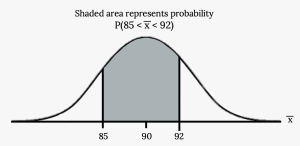
a. Find the probability that the sample mean is between 85 and 92.
- Let X = one value from the original unknown population. The probability question asks you to find a probability for the sample mean.
- Find P(85 < [latex]\overline{x}[/latex] < 92). Draw a graph.
b. Find the value that is two standard deviations above the expected value, 90, of the sample mean.
Using the TI-83, 83+, 84, 84+ Calculator
To find probabilities for means on the calculator, follow these steps.
2nd DISTR
2:normalcdf()
[latex]normalcdf\left(lower\text{ }value\text{ }of\text{ }the\text{ }area,\text{ }upper\text{ }value\text{ }of\text{ }the\text{ }area,\text{ }mean,\text{ }\frac{standard deviation}{\sqrt{sample size}}\right)[/latex]
where:
- mean is the mean of the original distribution
- standard deviation is the standard deviation of the original distribution
- sample size = n
Example
Using the graphing calculator for the previous problem:
An unknown distribution has a mean of 90 and a standard deviation of 15. Samples of size n = 25 are drawn randomly from the population. Find the probability that the sample mean is between 85 and 92.
Solution
Let X = one value from the original unknown population. The probability question asks you to find a probability for the sample mean.
Let [latex]\overline{X}[/latex] = the mean of a sample of size 25. Since μX = 90, σX = 15, and n = 25,
[latex]\overline{X}[/latex] ~ N[latex]\left(90\text{, }\frac{15}{\sqrt{25}}\right)[/latex].
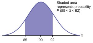
Find P(85 < [latex]\overline{x}[/latex] < 92). Draw a graph.
normalcdf(lower value, upper value, mean, standard error of the mean)
The parameter list is abbreviated (lower value, upper value, μ, [latex]\frac{\sigma }{\sqrt{n}}[/latex])
normalcdf(85,92,90,[latex]\frac{15}{\sqrt{25}}[/latex]) = 0.6997
Your Turn!
An unknown distribution has a mean of 45 and a standard deviation of eight. Samples of size n = 30 are drawn randomly from the population. Find the probability that the sample mean is between 42 and 50.
Solution
P(42 < [latex]\overline{x}[/latex] < 50) = [latex]\left(\text{42,50,45,}\frac{8}{\sqrt{30}}\right)[/latex] = 0.9797
Example
The length of time, in hours, it takes an “over 40” group of people to play one soccer match is normally distributed with a mean of two hours and a standard deviation of 0.5 hours. A sample of size n = 50 is drawn randomly from the population. Find the probability that the sample mean is between 1.8 hours and 2.3 hours.
Solution
Let X = the time, in hours, it takes to play one soccer match.
The probability question asks you to find a probability for the sample mean time, in hours, it takes to play one soccer match.
Let [latex]\overline{X}[/latex] = the mean time, in hours, it takes to play one soccer match.
If μX = _________, σX = __________, and n = ___________, then X ~ N(______, ______) by the central limit theorem for means.
μX = 2, σX = 0.5, n = 50, and X ~ N[latex]\left(\text{2, }\frac{0.5}{\sqrt{50}}\right)[/latex]
Find P(1.8 < [latex]\overline{x}[/latex] < 2.3). Draw a graph.
P(1.8 < [latex]\overline{x}[/latex] < 2.3) = 0.9977
normalcdf[latex]\left(1.\text{8,2}\text{.3,2,}\frac{.5}{\sqrt{50}}\right)[/latex] = 0.9977
The probability that the mean time is between 1.8 hours and 2.3 hours is 0.9977.
Your Turn!
The length of time taken on the SAT for a group of students is normally distributed with a mean of 2.5 hours and a standard deviation of 0.25 hours. A sample size of n = 60 is drawn randomly from the population. Find the probability that the sample mean is between two hours and three hours.
Solution
P(2 < [latex]\overline{x}[/latex] < 3) = normalcdf[latex]\left(\text{2, 3, 2}\text{.5, }\frac{0.25}{\sqrt{60}}\right)[/latex] = 1
Using the TI-83, 83+, 84, 84+ Calculator
To find percentiles for means on the calculator, follow these steps.
2nd DIStR
3: invNorm()
k = invNorm[latex]\left(\text{area to the left of }k\text{, mean,} \frac{standard deviation}{\sqrt{sample size}}\right)[/latex]
where:
- k = the kth percentile
- mean is the mean of the original distribution
- standard deviation is the standard deviation of the original distribution
- sample size = n
Example
In a recent study reported Oct. 29, 2012 on the Flurry Blog, the mean age of tablet users is 34 years. Suppose the standard deviation is 15 years. Take a sample of size n = 100.
- What are the mean and standard deviation for the sample mean ages of tablet users?
- What does the distribution look like?
- Find the probability that the sample mean age is more than 30 years (the reported mean age of tablet users in this particular study).
- Find the 95th percentile for the sample mean age (to one decimal place).
Solution
- Since the sample mean tends to target the population mean, we have μχ = μ = 34. The sample standard deviation is given by σχ = [latex]\frac{\sigma }{\sqrt{n}}[/latex] = [latex]\frac{15}{\sqrt{100}}[/latex] = [latex]\frac{15}{10}[/latex] = 1.5
- The central limit theorem states that for large sample sizes(n), the sampling distribution will be approximately normal.
- The probability that the sample mean age is more than 30 is given by P(Χ > 30) =
normalcdf(30,E99,34,1.5) = 0.9962 - Let k = the 95th percentile. k = invNorm[latex]\left(0.\text{95,34,}\frac{15}{\sqrt{100}}\right)[/latex] = 36.5
Your Turn!
In an article on Flurry Blog, a gaming marketing gap for men between the ages of 30 and 40 is identified. You are researching a startup game targeted at the 35-year-old demographic. Your idea is to develop a strategy game that can be played by men from their late 20s through their late 30s. Based on the article’s data, industry research shows that the average strategy player is 28 years old with a standard deviation of 4.8 years. You take a sample of 100 randomly selected gamers. If your target market is 29- to 35-year-olds, should you continue with your development strategy?
Solution
You need to determine the probability for men whose mean age is between 29 and 35 years of age wanting to play a strategy game.
P(29 < [latex]\overline{x}[/latex] < 35) = normalcdf[latex]\left(\text{29,35,28,}\frac{4.8}{\sqrt{100}}\right)[/latex] = 0.0186
You can conclude there is approximately a 1.9% chance that your game will be played by men whose mean age is between 29 and 35.
Example
The mean number of minutes for app engagement by a tablet user is 8.2 minutes. Suppose the standard deviation is one minute. Take a sample of 60.
- What are the mean and standard deviation for the sample mean number of app engagement by a tablet user?
- What is the standard error of the mean?
- Find the 90th percentile for the sample mean time for app engagement for a tablet user. Interpret this value in a complete sentence.
- Find the probability that the sample mean is between eight minutes and 8.5 minutes.
Solution
- [latex]{\mu }_{\overline{x}}=\mu =8.2\text{ }{\sigma }_{\overline{x}}=\frac{\sigma }{\sqrt{n}}=\frac{1}{\sqrt{60}}=0.13[/latex]
- This allows us to calculate the probability of sample means of a particular distance from the mean, in repeated samples of size 60.
- Let k = the 90th percentile
k =
invNorm[latex]\left(0.\text{90,8}\text{.2,}\frac{1}{\sqrt{60}}\right)[/latex] = 8.37. This value indicates that 90 percent of the average app engagement time for table users is less than 8.37 minutes. - P(8 < [latex]\overline{x}[/latex] < 8.5) =
normalcdf[latex]\left(\text{8,8}\text{.5,8}\text{.2,}\frac{1}{\sqrt{60}}\right)[/latex] = 0.9293
Your Turn!
Cans of a cola beverage claim to contain 16 ounces. The amounts in a sample are measured and the statistics are n = 34, [latex]\overline{x}[/latex] = 16.01 ounces. If the cans are filled so that μ = 16.00 ounces (as labeled) and σ = 0.143 ounces, find the probability that a sample of 34 cans will have an average amount greater than 16.01 ounces. Do the results suggest that cans are filled with an amount greater than 16 ounces?
Solution
We have P([latex]\overline{x}[/latex] > 16.01) = normalcdf[latex]\left(\text{16}\text{.01,E99,16,}\frac{0.143}{\sqrt{34}}\right)[/latex] = 0.3417. Since there is a 34.17% probability that the average sample weight is greater than 16.01 ounces, we should be skeptical of the company’s claimed volume. If I am a consumer, I should be glad that I am probably receiving free cola. If I am the manufacturer, I need to determine if my bottling processes are outside of acceptable limits.
Note
It is important for you to understand when to use the central limit theorem. If you are being asked to find the probability of the mean, use the clt for the mean. This also applies to percentiles for means. If you are being asked to find the probability of an individual value, do not use the clt. Use the distribution of its random variable.
Example
Suppose that a market research analyst for a cell phone company conducts a study of their customers who exceed the time allowance included on their basic cell phone contract; the analyst finds that for those people who exceed the time included in their basic contract, the excess time used follows an exponential distribution with a mean of 22 minutes.
Consider a random sample of 80 customers who exceed the time allowance included in their basic cell phone contract.
Let X = the excess time used by one INDIVIDUAL cell phone customer who exceeds his contracted time allowance.
X ∼ Exp[latex]\left(\frac{1}{22}\right)[/latex]. From previous chapters, we know that μ = 22 and σ = 22.
Let [latex]\overline{X}[/latex] = the mean excess time used by a sample of n = 80 customers who exceed their contracted time allowance.
[latex]\overline{X}[/latex] ~ N[latex]\left(\text{22, }\frac{\text{22}}{\sqrt{\text{80}}}\right)[/latex] by the central limit theorem for sample means
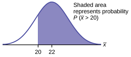
- Find the probability that the mean excess time used by the 80 customers in the sample is longer than 20 minutes. This is asking us to find P([latex]\overline{x}[/latex] > 20). Draw the graph.
- Suppose that one customer who exceeds the time limit for his cell phone contract is randomly selected. Find the probability that this individual customer’s excess time is longer than 20 minutes. This is asking us to find P(x > 20).
- Explain why the probabilities in parts a and b are different.
Solution
-
Find: P([latex]\overline{x}[/latex] > 20)
P([latex]\overline{x}[/latex] > 20) = 0.79199 using
normalcdf[latex]\left(\text{20,1E99,22,}\frac{\text{22}}{\sqrt{\text{80}}}\right)[/latex]The probability is 0.7919 that the mean excess time used is more than 20 minutes, for a sample of 80 customers who exceed their contracted time allowance.
 Reminder
1E99 = 1099 and –1E99 = –1099. Press the
EEkey for E. Or just use 1099 instead of 1E99. - Find P(x > 20). Remember to use the exponential distribution for an individual: [latex]X~Exp\left(\frac{1}{22}\right)[/latex].
[latex]P\left(x>20\right)\text{ = }{e}^{\left(-\left(\frac{1}{22}\right)\left(20\right)\right)}[/latex] or e(–0.04545(20)) = 0.4029
- P(x > 20) = 0.4029 but P([latex]\overline{x}[/latex] > 20) = 0.7919
- The probabilities are not equal because we use different distributions to calculate the probability for individuals and for means.
- When asked to find the probability of an individual value, use the stated distribution of its random variable; do not use the clt. Use the clt with the normal distribution when you are being asked to find the probability for a mean.
Using the clt to find percentiles
Find the 95th percentile for the sample mean excess time for samples of 80 customers who exceed their basic contract time allowances. Draw a graph.
Solution
Let k = the 95th percentile. Find k where P([latex]\overline{x}[/latex] < k) = 0.95
k = 26.0 using invNorm[latex]\left(\text{0}\text{.95,22},\frac{22}{\sqrt{80}}\right)[/latex] = 26.0
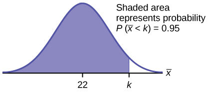
The 95th percentile for the sample mean excess time used is about 26.0 minutes for random samples of 80 customers who exceed their contractual allowed time.
Ninety five percent of such samples would have means under 26 minutes; only five percent of such samples would have means above 26 minutes.
Example
Based on data from the National Health Survey, women between the ages of 18 and 24 have an average systolic blood pressures (in mmHg) of 114.8 with a standard deviation of 13.1. Systolic blood pressure for women between the ages of 18 to 24 follows a normal distribution.
- If one woman from this population is randomly selected, find the probability that her systolic blood pressure is greater than 120.
- If 40 women from this population are randomly selected, find the probability that their mean systolic blood pressure is greater than 120.
- If the sample were four women between the ages of 18 to 24 and we did not know the original distribution, could the central limit theorem be used?
Solution
- P(x > 120) =
normalcdf(120,99,114.8,13.1) = 0.0272. There is about a 3% that the randomly selected woman will have systolic blood pressure greater than 120. - P([latex]\overline{x}[/latex] > 120) =
normalcdf[latex]\left(\text{120,114}\text{.8,}\frac{\text{13}\text{.1}}{\sqrt{\text{40}}}\right)[/latex] = 0.006. There is only a 0.6% chance that the average systolic blood pressure for the randomly selected group is greater than 120. - The central limit theorem could not be used if the sample size were four and we did not know the original distribution was normal. The sample size would be too small.
Your Turn!
According to Boeing data, the 757 airliner carries 200 passengers and has doors with a mean height of 72 inches. Assume for a certain population of men we have a mean of 69.0 inches and a standard deviation of 2.8 inches.
- What mean doorway height would allow 95% of men to enter the aircraft without bending?
- Assume that half of the 200 passengers are men. What mean doorway height satisfies the condition that there is a 0.95 probability that this height is greater than the mean height of 100 men?
- For engineers designing the 757, which result is more relevant: the height from part a or part b? Why?
Solution
- We know that μx = μ = 69 and we have σx = 2.8. The height of the doorway is found to be
invNorm(0.95,69,2.8) = 73.61 - We know that μx = μ = 69 and we have σx = 0.28. So,
invNorm(0.95,69,0.28) = 69.49 - When designing the doorway heights, we need to incorporate as much variability as possible in order to accommodate as many passengers as possible. Therefore, we need to use the result based on part a.
References
Baran, Daya. “20 Percent of Americans Have Never Used Email.” WebGuild, 2010. Available online at http://www.webguild.org/20080519/20-percent-of-americans-have-never-used-email (accessed May 17, 2013).
Data from The Flurry Blog, 2013. Available online at http://blog.flurry.com (accessed May 17, 2013).
Data from the United States Department of Agriculture.
Media Attributions
- Private: 6.2.1
- Private: 6.4
- Figure 7.2 © OpenStax Introductory Statistics is licensed under a CC BY (Attribution) license
As the number of trials in a probability experiment increases, the difference between the theoretical probability of an event and the relative frequency probability approaches zero.
Given a random variable (RV) with known mean [latex]\mu[/latex] and known standard deviation σ. We are sampling with size n and we are interested in two new RVs - the sample mean, [latex]\overline{X}[/latex], and the sample sum, [latex]\Sigma X[/latex].
If the size n of the sample is sufficiently large, then [latex]\overline{X}~N\left(\mu \text{,}\frac{\sigma }{\sqrt{n}}\right)[/latex] and [latex]\Sigma X~N\left(n\mu ,\sqrt{n}\sigma \right)[/latex]. If the size n of the sample is sufficiently large, then the distribution of the sample means and the distribution of the sample sums will approximate a normal distribution regardless of the shape of the population. The mean of the sample means will equal the population mean and the mean of the sample sums will equal n times the population mean. The standard deviation of the distribution of the sample means, [latex]\frac{\sigma }{\sqrt{n}}[/latex], is called the standard error of the mean.
a continuous random variable (RV) with pdf [latex]f\text{(}x\text{)}=\frac{1}{\sigma \sqrt{2\pi }}{e}^{–{\left(x–\mu \right)}^{2}/2{\sigma }^{2}}[/latex], where μ is the mean of the distribution and σ is the standard deviation, notation: X ~ N(μ,σ). If μ = 0 and σ = 1, the RV is called the standard normal distribution.
a number that describes the central tendency of the data; there are a number of specialized averages, including the arithmetic mean, weighted mean, median, mode, and geometric mean.
the standard deviation of the distribution of the sample means, or [latex]\frac{\sigma }{\sqrt{n}}[/latex].
