Chapter 11: The Chi-Square Distribution
11.3 Test of Independence
Learning Objectives
By the end of this section, the student should be able to:
- calculate the test of independence and determines whether two factors are independent or not
Tests of independence involve using a contingency table of observed (data) values.
The test statistic for a test of independence is similar to that of a goodness-of-fit test:
where:
- O = observed values
- E = expected values
- i = the number of rows in the table
- j = the number of columns in the table
There are [latex]i\cdot j[/latex] terms of the form [latex]\frac{{\left(O–E\right)}^{2}}{E}[/latex].
A test of independence determines whether two factors are independent or not. You first encountered the term independence in Probability Topics. As a review, consider the following example.
Note
The expected value for each cell needs to be at least five in order for you to use this test.
Example
Suppose A = a speeding violation in the last year and B = a cell phone user while driving. If A and B are independent then P(A AND B) = P(A)P(B). A AND B is the event that a driver received a speeding violation last year and also used a cell phone while driving. Suppose, in a study of drivers who received speeding violations in the last year and who used cell phones while driving, that 755 people were surveyed. Out of the 755, 70 had a speeding violation and 685 did not; 305 used cell phones while driving and 450 did not.
Let y = expected number of drivers who used a cell phone while driving and received speeding violations.
If A and B are independent, then P(A AND B) = P(A)P(B). By substitution,
[latex]\frac{y}{755}=\left(\frac{70}{755}\right)\left(\frac{305}{755}\right)[/latex]
Solve for y: y = [latex]\frac{\left(70\right)\left(305\right)}{755}=28.3[/latex]
About 28 people from the sample are expected to use cell phones while driving and to receive speeding violations.
In a test of independence, we state the null and alternative hypotheses in words. Since the contingency table consists of two factors, the null hypothesis states that the factors are independent and the alternative hypothesis states that they are not independent (dependent). If we do a test of independence using the example, then the null hypothesis is:
H0: Being a cell phone user while driving and receiving a speeding violation are independent events.
If the null hypothesis were true, we would expect about 28 people to use cell phones while driving and to receive a speeding violation.
The test of independence is always right-tailed because of the calculation of the test statistic. If the expected and observed values are not close together, then the test statistic is very large and way out in the right tail of the chi-square curve, as it is in a goodness-of-fit.
The number of degrees of freedom for the test of independence is:
df = (number of columns – 1)(number of rows – 1)
The following formula calculates the expected number (E):
[latex]E=\frac{\text{(row total)(column total)}}{\text{total number surveyed}}[/latex]
Your Turn!
A sample of 300 students is taken. Of the students surveyed, 50 were music students, while 250 were not. Ninety-seven were on the honor roll, while 203 were not. If we assume being a music student and being on the honor roll are independent events, what is the expected number of music students who are also on the honor roll?
Solution
About 16 students are expected to be music students and on the honor roll.
Example
In a volunteer group, adults 21 and older volunteer from one to nine hours each week to spend time with a disabled senior citizen. The program recruits among community college students, four-year college students, and nonstudents. In [link] is a sample of the adult volunteers and the number of hours they volunteer per week.
| Type of Volunteer | 1–3 Hours | 4–6 Hours | 7–9 Hours | Row Total |
|---|---|---|---|---|
| Community College Students | 111 | 96 | 48 | 255 |
| Four-Year College Students | 96 | 133 | 61 | 290 |
| Nonstudents | 91 | 150 | 53 | 294 |
| Column Total | 298 | 379 | 162 | 839 |
Is the number of hours volunteered independent of the type of volunteer?
Solution
The observed table and the question at the end of the problem, “Is the number of hours volunteered independent of the type of volunteer?” tell you this is a test of independence. The two factors are number of hours volunteered and type of volunteer. This test is always right-tailed.
H0: The number of hours volunteered is independent of the type of volunteer.
Ha: The number of hours volunteered is dependent on the type of volunteer.
The expected results are in [link].
| Type of Volunteer | 1-3 Hours | 4-6 Hours | 7-9 Hours |
|---|---|---|---|
| Community College Students | 90.57 | 115.19 | 49.24 |
| Four-Year College Students | 103.00 | 131.00 | 56.00 |
| Nonstudents | 104.42 | 132.81 | 56.77 |
For example, the calculation for the expected frequency for the top left cell is
[latex]E=\frac{\left(\text{row total}\right)\left(\text{column total}\right)}{\text{total number surveyed}}=\frac{\left(255\right)\left(298\right)}{839}=90.57[/latex]
Calculate the test statistic:χ2 = 12.99 (calculator or computer)
Distribution for the test:[latex]{\chi }_{4}^{2}[/latex]
df = (3 columns – 1)(3 rows – 1) = (2)(2) = 4
Graph:
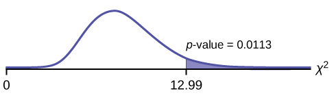
Probability statement:p-value=P(χ2 > 12.99) = 0.0113
Compare α and the p-value: Since no α is given, assume α = 0.05. p-value = 0.0113. α > p-value.
Make a decision: Since α > p-value, reject H0. This means that the factors are not independent.
Conclusion: At a 5% level of significance, from the data, there is sufficient evidence to conclude that the number of hours volunteered and the type of volunteer are dependent on one another.
For the example in [link], if there had been another type of volunteer, teenagers, what would the degrees of freedom be?
Press the MATRX key and arrow over to EDIT. Press 1:[A]. Press 3 ENTER 3 ENTER. Enter the table values by row from [link]. Press ENTER after each. Press 2nd QUIT. Press STAT and arrow over to TESTS. Arrow down to C:χ2-TEST. Press ENTER. You should see Observed:[A] and Expected:[B]. Arrow down to Calculate. Press ENTER. The test statistic is 12.9909 and the p-value = 0.0113. Do the procedure a second time, but arrow down to Draw instead of calculate.
Your Turn!
The Bureau of Labor Statistics gathers data about employment in the United States. A sample is taken to calculate the number of U.S. citizens working in one of several industry sectors over time. [link] shows the results:
| Industry Sector | 2000 | 2010 | 2020 | Total |
|---|---|---|---|---|
| Nonagriculture wage and salary | 13,243 | 13,044 | 15,018 | 41,305 |
| Goods-producing, excluding agriculture | 2,457 | 1,771 | 1,950 | 6,178 |
| Services-providing | 10,786 | 11,273 | 13,068 | 35,127 |
| Agriculture, forestry, fishing, and hunting | 240 | 214 | 201 | 655 |
| Nonagriculture self-employed and unpaid family worker | 931 | 894 | 972 | 2,797 |
| Secondary wage and salary jobs in agriculture and private household industries | 14 | 11 | 11 | 36 |
| Secondary jobs as a self-employed or unpaid family worker | 196 | 144 | 152 | 492 |
| Total | 27,867 | 27,351 | 31,372 | 86,590 |
We want to know if the change in the number of jobs is independent of the change in years. State the null and alternative hypotheses and the degrees of freedom.
Solution
H0 : The number of jobs is independent of the year.
Ha : The number of jobs is dependent on the year.
df = 12

Press the MATRX key and arrow over to EDIT. Press 1:[A]. Press 3 ENTER 3 ENTER. Enter the table values by row. Press ENTER after each. Press 2nd QUIT. Press STAT and arrow over to TESTS. Arrow down to C:χ2-TEST. Press ENTER. You should see Observed:[A] and Expected:[B]. Arrow down to Calculate. Press ENTER. The test statistic is 227.73 and the p−value = 5.90E – 42 = 0. Do the procedure a second time but arrow down to Draw instead of calculate.
Example
De Anza College is interested in the relationship between anxiety level and the need to succeed in school. A random sample of 400 students took a test that measured anxiety level and the need to succeed in school. [link] shows the results. De Anza College wants to know if anxiety level and need to succeed in school are independent events.
| Need to Succeed in School | High
Anxiety |
Med-high
Anxiety |
Medium
Anxiety |
Med-low
Anxiety |
Low
Anxiety |
Row Total |
|---|---|---|---|---|---|---|
| High Need | 35 | 42 | 53 | 15 | 10 | 155 |
| Medium Need | 18 | 48 | 63 | 33 | 31 | 193 |
| Low Need | 4 | 5 | 11 | 15 | 17 | 52 |
| Column Total | 57 | 95 | 127 | 63 | 58 | 400 |
a. How many high anxiety level students are expected to have a high need to succeed in school?
Solution
a. The column total for a high anxiety level is 57. The row total for high need to succeed in school is 155. The sample size or total surveyed is 400.
[latex]E=\frac{\text{(row total)(column total)}}{\text{total surveyed}}=\frac{155\cdot 57}{400}=22.09[/latex]
The expected number of students who have a high anxiety level and a high need to succeed in school is about 22.
b. If the two variables are independent, how many students do you expect to have a low need to succeed in school and a med-low level of anxiety?
Solution
b. The column total for a med-low anxiety level is 63. The row total for a low need to succeed in school is 52. The sample size or total surveyed is 400.
c. [latex]E=\frac{\text{(row total)(column total)}}{\text{total surveyed}}[/latex] = ________
Solution
c. [latex]E=\frac{\text{(row total)(column total)}}{\text{total surveyed}}=8.19[/latex]
d. The expected number of students who have a med-low anxiety level and a low need to succeed in school is about ________.
Solution
d. 8
Your Turn!
Refer back to the information in [link]. How many service providing jobs are there expected to be in 2020? How many nonagriculture wage and salary jobs are there expected to be in 2020?
Solution
12,727, 14,965
References
DiCamilo, Mark, Mervin Field. “Most Californians See a Direct Linkage between Obesity and Sugary Sodas. Two in Three Voters Support Taxing Sugar-Sweetened Beverages If Proceeds Are Tied to Improving School Nutrition and Physical Activity Programs.” The Field Poll, released Feb. 14, 2013. Available online at http://field.com/fieldpollonline/subscribers/Rls2436.pdf (accessed May 24, 2013).
Harris Interactive. “Favorite Flavor of Ice Cream.” Available online at http://www.statisticbrain.com/favorite-flavor-of-ice-cream (accessed May 24, 2013)
“Youngest Online Entrepreneurs List.” Available online at http://www.statisticbrain.com/youngest-online-entrepreneur-list (accessed May 24, 2013).
