Chapter 5: Continuous Random Variables
5.1 Continuous Probability Functions
Learning Objectives
By the end of this section, students will be able to:
- describe the properties of continuous probability distributions.
Properties of Continuous Probability Distributions
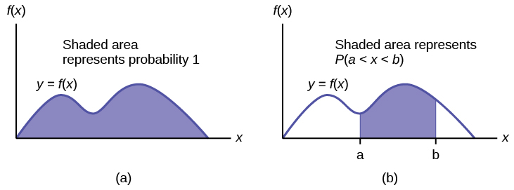
The graph of a continuous probability distribution is a curve. Probability is represented by area under the curve.
The curve is called the probability density function (abbreviated as pdf). We use the symbol [latex]f(x)[/latex] to represent the curve. [latex]f(x)[/latex] is the function that corresponds to the graph; we use the density function [latex]f(x)[/latex] to draw the graph of the probability distribution.
Area under the curve is given by a different function called the cumulative distribution function (abbreviated as cdf). The cumulative distribution function is used to evaluate probability as area.
- The outcomes are measured, not counted.
- The entire area under the curve and above the x-axis is equal to one.
- Probability is found for intervals of x values rather than for individual [latex]x[/latex] values.
- [latex]P(c \lt x \lt d)[/latex] is the probability that the random variable [latex]X[/latex] is in the interval between the values [latex]c[/latex] and [latex]d[/latex]. [latex]P(c \lt x \lt d)[/latex] is the area under the curve, above the x-axis, to the right of [latex]c[/latex] and the left of [latex]d[/latex].
- [latex]P(x = c) = 0[/latex] The probability that x takes on any single individual value is zero. The area below the curve, above the x-axis, and between [latex]x = c[/latex] and [latex]x = c[/latex] has no width, and therefore no area (area = 0). Since the probability is equal to the area, the probability is also zero.
- [latex]P(c \lt x \lt d)[/latex] is the same as [latex]P(c \le x \le d)[/latex] because probability is equal to area.
We will find the area that represents probability by using geometry, formulas, technology, or probability tables. In general, calculus is needed to find the area under the curve for many probability density functions. When we use formulas to find the area in this textbook, the formulas were found by using the techniques of integral calculus. However, because most students taking this course have not studied calculus, we will not be using calculus in this textbook.
There are many continuous probability distributions. When using a continuous probability distribution to model probability, the distribution used is selected to model and fit the particular situation in the best way.
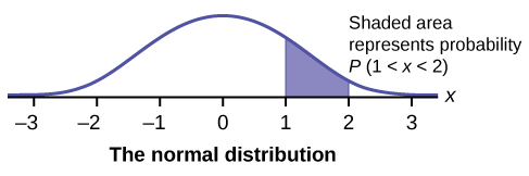
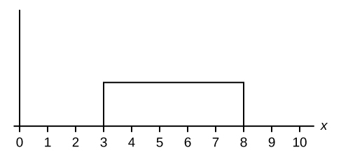
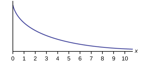
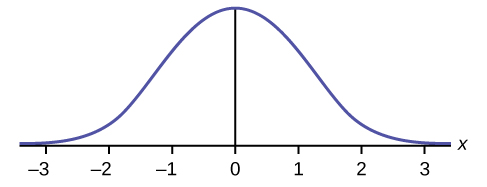
In this chapter and the next, we will study the uniform distribution, the exponential distribution, and the normal distribution. The following graphs illustrate these distributions.

Continuous Probability Functions
We begin by defining a continuous probability density function. We use the function notation [latex]f(x)[/latex]. Intermediate algebra may have been your first formal introduction to functions. In the study of probability, the functions we study are special. We define the function [latex]f(x)[/latex] so that the area between it and the x-axis is equal to a probability. Since the maximum probability is one, the maximum area is also one. For continuous probability distributions, PROBABILITY = AREA.
Example
Consider the function [latex]f(x) = \frac{1}{20}[/latex] for [latex]0 \le x \le 20[/latex]. [latex]x =[/latex] a real number. The graph of [latex]f(x) = \frac{1}{20}[/latex] is a horizontal line. However, since [latex]0 \le x \le 20[/latex], [latex]f(x)[/latex] is restricted to the portion between [latex]x = 0[/latex] and [latex]x = 20[/latex], inclusive.
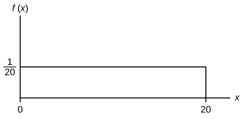
[latex]f(x)= \frac{1}{20}[/latex]for [latex]0 \le x \le 20[/latex].
The graph of [latex]f(x) = \frac{1}{20}[/latex] is a horizontal line segment when [latex]0 \le x \le 20[/latex].
The area between [latex]f(x) = \frac{1}{20}[/latex] where [latex]0 \le x \le 20[/latex] and the x-axis is the area of a rectangle with [latex]\text{base} = 20[/latex] and [latex]\text{height} = \frac{1}{20}[/latex].
Suppose we want to find the area between [latex]f(x) = \frac{1}{20}[/latex] and the x-axis where [latex]0 \lt x \lt 2[/latex].
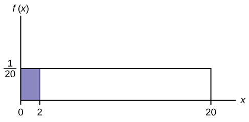
[latex]\text{AREA}=(2–0)(\frac{1}{20})=0.1[/latex]
[latex](2–0)=2=\text{base of a rectangle}[/latex]
Reminder: area of a rectangle = (base)(height).
The area corresponds to a probability. The probability that [latex]x[/latex] is between zero and two is 0.1, which can be written mathematically as [latex]P(0 \lt x \lt 2) = P(x \lt 2) = 0.1[/latex].
Suppose we want to find the area between [latex]f(x) = \frac{1}{20}[/latex] and the x-axis where [latex]4 \lt x \lt 15[/latex].
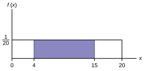
[latex]\text{AREA} = (15 - 4)(\frac{1}{20}) = 0.55[/latex]
The area corresponds to the probability [latex]P(4 \lt x \lt 15) = 0.55[/latex].
Suppose we want to find [latex]P(x = 15)[/latex]. On an x-y graph, [latex]x = 15[/latex] is a vertical line. A vertical line has no width (or zero width). Therefore, [latex]P(x = 15) = (\text{base})(\text{height}) = (0)(\frac{1}{20}) = 0[/latex].
[latex]P(X \le x)[/latex] (can be written as [latex]P(X \lt x)[/latex] for continuous distributions) is called the cumulative distribution function or CDF. Notice the “less than or equal to” symbol. We can use the CDF to calculate [latex]P(X > x)[/latex]. The CDF gives “area to the left” and [latex]P(X > x)[/latex] gives “area to the right.” We calculate [latex]P(X > x)[/latex] for continuous distributions as follows: [latex]P(X > x) = 1 – P (X \lt x)[/latex].
Label the graph with [latex]f(x)[/latex] and [latex]x[/latex]. Scale the x and y axes with the maximum x and y values. [latex]f(x) = \frac{1}{20}[/latex], [latex]0 \lt x \lt 20[/latex].
To calculate the probability that x is between two values, look at the following graph. Shade the region between [latex]x = 2.3[/latex] and [latex]x = 12.7[/latex]. Then calculate the shaded area of a rectangle.
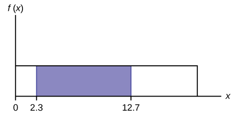
[latex]P(2.3 \lt x \lt 12.7 ) = ( \text{base} ) ( \text{height} ) = ( 12.7-2.3 ) ( \frac{1}{20} ) = 0.52[/latex]
Your Turn!
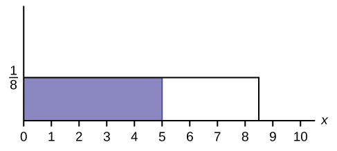
Consider the function [latex]f(x) = \frac{1}{8}[/latex] for [latex]0 \le x \le 8[/latex]. Draw the graph of [latex]f(x)[/latex] and find [latex]P(2.5 \lt x \lt 7.5)[/latex].
Solution

[latex]P (2.5 \lt x \lt 7.5) = 0.625[/latex]
Section 5.1 Review
The probability density function (pdf) is used to describe probabilities for continuous random variables. The area under the density curve between two points corresponds to the probability that the variable falls between those two values. In other words, the area under the density curve between points [latex]a[/latex] and [latex]b[/latex] is equal to [latex]P(a \lt x \lt b)[/latex]. The cumulative distribution function (cdf) gives the probability as an area. If [latex]X[/latex] is a continuous random variable, the probability density function (pdf), [latex]f(x)[/latex], is used to draw the graph of the probability distribution. The total area under the graph of f(x) is one. The area under the graph of [latex]f(x)[/latex] and between values a and b gives the probability [latex]P(a \lt x \lt b)[/latex].
The cumulative distribution function (cdf) of [latex]X[/latex] is defined by [latex]P (X \le x)[/latex]. It is a function of [latex]x[/latex] that gives the probability that the random variable is less than or equal to [latex]x[/latex].
Formula Review
Probability density function (pdf) [latex]f(x)[/latex]:
- [latex]f(x) \ge 0[/latex]
- The total area under the curve [latex]f(x)[/latex] is one.
Cumulative distribution function (cdf): [latex]P(X \le x)[/latex]
Section 5.1 Practice
Which type of distribution does the graph illustrate?
Solution
Uniform Distribution
Which type of distribution does the graph illustrate?
Which type of distribution does the graph illustrate?
Solution
Normal Distribution
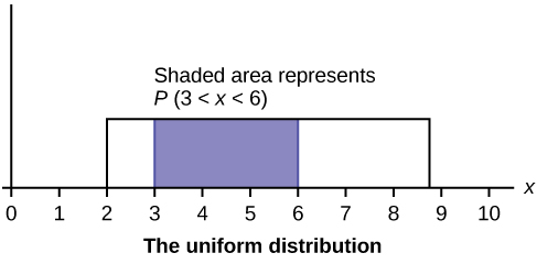
What does the shaded area represent? [latex]P(\underline{\hspace{2cm}} \lt x \lt \underline{\hspace{2cm}})[/latex]
What does the shaded area represent? [latex]P(\underline{\hspace{2cm}} \lt x \lt \underline{\hspace{2cm}})[/latex]
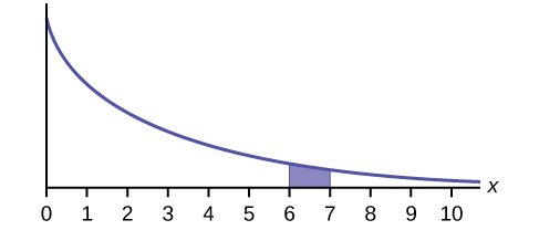
Solution
[latex]P(6 \lt x \lt 7)[/latex]
For a continuous probability distribution, [latex]0 \le x \le 15[/latex]. What is [latex]P(x > 15)[/latex]?
What is the area under [latex]f(x)[/latex] if the function is a continuous probability density function?
Solution
one
For a continuous probability distribution, [latex]0 \le x \le 10[/latex]. What is [latex]P(x = 7)[/latex]?
A continuous probability function is restricted to the portion between [latex]x = 0 \text{ and } 7[/latex]. What is [latex]P(x = 10)[/latex]?
Solution
zero
[latex]f(x)[/latex] for a continuous probability function is [latex]\frac{1}{5}[/latex], and the function is restricted to [latex]0 \le x \le 5[/latex]. What is [latex]P(x \lt 0)[/latex]?
[latex]f(x)[/latex], a continuous probability function, is equal to [latex]\frac{1}{12}[/latex], and the function is restricted to [latex]0 \le x \le 12[/latex]. What is [latex]P (0 \lt x \lt 12)[/latex]?
Solution
one
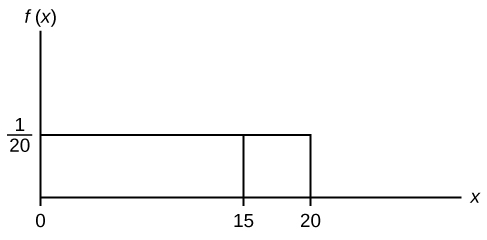
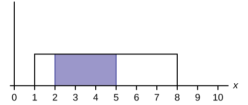
Find the probability that [latex]x[/latex] falls in the shaded area.

Find the probability that [latex]x[/latex] falls in the shaded area.
Solution
0.625
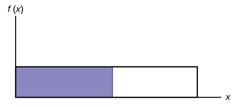
Find the probability that [latex]x[/latex] falls in the shaded area.

[latex]f(x)[/latex], a continuous probability function, is equal to [latex]\frac{1}{3}[/latex] and the function is restricted to [latex]1\le x \le 4[/latex]. Describe [latex]P (x>\frac{3}{2})[/latex].
Solution
The probability is equal to the area from [latex]x= \frac{3}{2}[/latex] to [latex]x = 4[/latex] above the x-axis and up to [latex]f(x) =\frac{1}{3}[/latex].
Consider the following experiment. You are one of 100 people enlisted to take part in a study to determine the percent of nurses in America with an R.N. (registered nurse) degree. You ask nurses if they have an R.N. degree. The nurses answer “yes” or “no.” You then calculate the percentage of nurses with an R.N. degree. You give that percentage to your supervisor.
- What part of the experiment will yield discrete data?
- What part of the experiment will yield continuous data?
When age is rounded to the nearest year, do the data stay continuous, or do they become discrete? Why?
Solution
Age is a measurement, regardless of the accuracy used.
a continuous random variable (RV) that has equally likely outcomes over the domain, a < x < b; it is often referred to as the rectangular distribution because the graph of the pdf has the form of a rectangle. Notation: X ~ U(a,b). The mean is μ = [latex]\frac{a+b}{2}[/latex] and the standard deviation is [latex]\sigma =\sqrt{\frac{{\left(b-a\right)}^{2}}{12}}[/latex]. The probability density function is f(x) = [latex]\frac{1}{b-a}[/latex] for a < x < b or a ≤ x ≤ b. The cumulative distribution is P(X ≤ x) = [latex]\frac{x-a}{b-a}[/latex].
a continuous random variable (RV) that appears when we are interested in the intervals of time between some random events, for example, the length of time between emergency arrivals at a hospital; the notation is X ~ Exp(m). The mean is μ = 1m and the standard deviation is σ = 1m. The probability density function is f(x) = me−mx, x ≥ 0 and the cumulative distribution function is P(X ≤ x) = 1 − e−mx.
