Chapter 4: Discrete Random Variables
4.6 Poisson Distribution
Learning Objectives
By the end of this section, the student should be able to:
- Identify the components of a Poisson experiment
- Use the formulas for a Poisson random variable to compute the mean, variance, and standard deviation
There are two main characteristics of a Poisson experiment.
- The Poisson probability distribution gives the probability of a number of events occurring in a fixed interval of time or space if these events happen with a known average rate and independently of the time since the last event. For example, a book editor might be interested in the number of words spelled incorrectly in a particular book. It might be that, on the average, there are five words spelled incorrectly in 100 pages. The interval is the 100 pages.
- The number of events occurring has a constant average and the events are independent of the “time” since the last event. Continuing the book example, the average number of misspelled words is 5, and finding a word that is misspelled does not influence the page on which the next misspelled word lies. Additionally, two events shouldn’t occur simultaneously.
The Poisson distribution is frequently used for experiments where there are a large number of possible but rare events. For instance, the Poisson distribution may be used to approximate the binomial if the probability of success is “small” (such as 0.01) and the number of trials is “large” (such as 1,000). You will verify the relationship in the homework exercises.
The random variable X = the number of occurrences in the interval of interest. Because the average per interval is constant, we can find the average for any size interval by scaling to the size of the interval.
Example
The average number of loaves of bread put on a shelf in a bakery in a half-hour period is 12. Of interest is the number of loaves of bread put on the shelf in five minutes, selected randomly. The time interval of interest is five minutes. What is the probability that the number of loaves put on the shelf in five minutes is three?
Let [latex]X =[/latex] the number of loaves of bread put on the shelf in five minutes. If the average number of loaves put on the shelf in 30 minutes (half-hour) is 12, then the average number of loaves put on the shelf in five minutes is [latex]\left(\frac{5}{30}\right)[/latex](12) = 2 loaves of bread.
The probability question asks you to find [latex]P(X = 3)[/latex].
Your Turn!
You notice that a news reporter says “uh,” on average, two times per broadcast. What is the probability that the news reporter says “uh” more than two times per broadcast.
This is a Poisson problem because you are interested in knowing the number of times the news reporter says “uh” during a broadcast.
a. What is the interval of interest?
Solution
a. one broadcast
b. What is the average number of times the news reporter says “uh” during one broadcast?
Solution
b. 2
c. Let X = ____________. What values does X take on?
Solution
c. Let X = the number of times the news reporter says “uh” during one broadcast.
x = 0, 1, 2, 3, …
d. The probability question is P(______).
Solution
d. P(x > 2)
Your Turn!
An emergency room at a particular hospital gets an average of five patients per hour. A doctor wants to know the probability that the ER gets more than five patients per hour. Give the reasons why this would be a Poisson distribution.
Your Turn!
The average number of fish caught in an hour is eight. Of interest is the number of fish caught in 15 minutes. What is the average number of fish caught in 15 minutes?
Notation and Mean
The notation for the Poisson Probability Distribution function is [latex]P[/latex], and we denote “X is a random variable with a Poisson probability distribution as [latex]X \sim P(\lambda)[/latex]. The parameter is [latex]\lambda[/latex], which is also the mean [latex]\mu[/latex]. So, we may also write [latex]X \sim P(\mu)[/latex].
The mean is given as part of a Poisson experiment, [latex]\mu = \lambda[/latex].
The formula for the variance is [latex]\sigma^2 = \lambda = \mu[/latex], that is, the average is also the variance of a Poisson random variable.
The formula for the standard deviation is [latex]\sigma = \sqrt{\lambda}[/latex].
Note
To compute Poisson probabilities on a graphing calculator, go into 2nd DISTR. The syntax for the instructions are as follows. The TI calculators use λ (lambda) for the mean.
To calculate [latex]P(X = x)[/latex]: poissonpdf([latex]\lambda[/latex], x).
To calculate [latex]P(X \leq x)[/latex]: poissoncdf([latex]\lambda[/latex], x).
If you wanted to instead find [latex]P(X>x)[/latex], use 1 – poissoncdf([latex]\lambda,x[/latex]).
In Excel, both geometric probabilities are computed using POISSON.DIST(x, [latex]\lambda[/latex], True/False), where False computes [latex]P(X=x)[/latex] and is equivalent to poissonpdf, and True computes [latex]P(X \leq x)[/latex] and is equivalent to poissoncdf.
Example
Leah’s school email receives an average of six emails between 8 a.m. and 10 a.m. each day. What is the probability that Leah receives more than one email in the next 15 minutes?
Let [latex]X =[/latex] the number of emails Leah receives in 15 minutes. (The interval of interest is 15 minutes or [latex]\frac{1}{4}[/latex] hour.)
x = 0, 1, 2, 3, …
If Leah receives, on the average, six emails in two hours, and there are eight 15 minute intervals in two hours, then Leah receives
[latex]\left(\frac{1}{8}\right)(6) = 0.75[/latex] emails in 15 minutes, on average. So, [latex]\lambda = \mu = 0.75[/latex] for this problem, and [latex]X \sim P(0.75)[/latex].
Find [latex]P(X > 1)[/latex]: (calculator or computer)
- Press 1 – and then press 2nd DISTR.
- Arrow down to poissoncdf(. Press ENTER.
- Enter .75,1).
- The result is [latex]P(X > 1) = 0.1734.[/latex]
The probability that Leah receives more than one email in the next 15 minutes is about 0.1734:
The graph of [latex]X \sim P(0.75)[/latex] is:
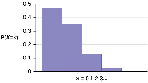
The y-axis contains the probability of x where X = the number of emails in 15 minutes.
Your Turn!
Atlanta’s Hartsfield-Jackson International Airport is the busiest airport in the world. On average there are 2,500 arrivals and departures each day.
- How many airplanes arrive and depart the airport per hour?
- What is the probability that there are exactly 100 arrivals and departures in one hour?
- What is the probability that there are at most 100 arrivals and departures in one hour?
Example
According to Baydin, an email management company, an email user gets, on average, 147 emails per day. Let [latex]X=[/latex] the number of emails an email user receives per day. The discrete random variable [latex]X[/latex] takes on the values [latex]x= 0, 1, 2, \ldots[/latex]. The random variable [latex]X[/latex] has a Poisson distribution: [latex]X \sim P(147)[/latex]. The mean is 147 emails.
- What is the probability that an email user receives exactly 160 emails per day?
- What is the probability that an email user receives at most 160 emails per day?
- What is the standard deviation?
Solution
- [latex]P(x = 160)[/latex] = poissonpdf(147, 160) ≈ 0.0180
- [latex]P(x \leq 160)[/latex] = poissoncdf(147, 160) ≈ 0.8666
- Standard Deviation = [latex]\sigma =\sqrt{\mu }=\sqrt{147}\approx 12.1244[/latex]
Your Turn!
According to a recent poll by the Pew Internet Project, girls between the ages of 14 and 17 send an average of 187 text messages each day. Let X = the number of texts that a girl aged 14 to 17 sends per day. The discrete random variable X takes on the values x = 0, 1, 2 …. The random variable X has a Poisson distribution: X ~ P(187). The mean is 187 text messages.
- What is the probability that a teen girl sends exactly 175 texts per day?
- What is the probability that a teen girl sends at most 150 texts per day?
- What is the standard deviation?
The Poisson distribution can be used to approximate probabilities for a binomial distribution. The Poisson approximation to a binomial distribution was commonly used in the days before technology made both values very easy to calculate.
Let [latex]n[/latex] represent the number of binomial trials and let [latex]p[/latex] represent the probability of a success for each trial. If [latex]n[/latex] is large enough and [latex]p[/latex] is small enough then the Poisson approximates the binomial very well. In general, [latex]n[/latex] is considered “large enough” if it is greater than or equal to 20. The probability [latex]p[/latex] from the binomial distribution should be less than or equal to 0.05. When the Poisson is used to approximate the binomial, we use the binomial mean [latex]\mu = np[/latex].
Example
On May 13, 2013, starting at 4:30 PM, the probability of low seismic activity for the next 48 hours in Alaska was reported as about 1.02%. Use this information for the next 200 days to find the probability that there will be low seismic activity in ten of the next 200 days. Use both the binomial and Poisson distributions to calculate the probabilities. Are they similar?
Your Turn!
On May 13, 2013, starting at 4:30 PM, the probability of moderate seismic activity for the next 48 hours in the Kuril Islands off the coast of Japan was reported at about 1.43%. Use this information for the next 100 days to find the probability that there will be low seismic activity in five of the next 100 days. Use both the binomial and Poisson distributions to calculate the probabilities. Are they close?
References
“ATL Fact Sheet,” Department of Aviation at the Hartsfield-Jackson Atlanta International Airport, 2013. Available online at http://www.atlanta-airport.com/Airport/ATL/ATL_FactSheet.aspx (accessed May 15, 2013).
Center for Disease Control and Prevention. “Teen Drivers: Fact Sheet,” Injury Prevention & Control: Motor Vehicle Safety, October 2, 2012. Available online at http://www.cdc.gov/Motorvehiclesafety/Teen_Drivers/teendrivers_factsheet.html (accessed May 15, 2013).
“Children and Childrearing,” Ministry of Health, Labour, and Welfare. Available online at http://www.mhlw.go.jp/english/policy/children/children-childrearing/index.html (accessed May 15, 2013).
“Eating Disorder Statistics,” South Carolina Department of Mental Health, 2006. Available online at http://www.state.sc.us/dmh/anorexia/statistics.htm (accessed May 15, 2013).
“Giving Birth in Manila: The maternity ward at the Dr Jose Fabella Memorial Hospital in Manila, the busiest in the Philippines, where there is an average of 60 births a day,” theguardian, 2013. Available online at http://www.theguardian.com/world/gallery/2011/jun/08/philippines-health#/?picture=375471900&index=2 (accessed May 15, 2013).
“How Americans Use Text Messaging,” Pew Internet, 2013. Available online at http://pewinternet.org/Reports/2011/Cell-Phone-Texting-2011/Main-Report.aspx (accessed May 15, 2013).
Lenhart, Amanda. “Teens, Smartphones & Testing: Texting volume is up while the frequency of voice calling is down. About one in four teens say they own smartphones,” Pew Internet, 2012. Available online at http://www.pewinternet.org/~/media/Files/Reports/2012/PIP_Teens_Smartphones_and_Texting.pdf (accessed May 15, 2013).
“One born every minute: the maternity unit where mothers are THREE to a bed,” MailOnline. Available online at http://www.dailymail.co.uk/news/article-2001422/Busiest-maternity-ward-planet-averages-60-babies-day-mothers-bed.html (accessed May 15, 2013).
Vanderkam, Laura. “Stop Checking Your Email, Now.” CNNMoney, 2013. Available online at http://management.fortune.cnn.com/2012/10/08/stop-checking-your-email-now/ (accessed May 15, 2013).
“World Earthquakes: Live Earthquake News and Highlights,” World Earthquakes, 2012. http://www.world-earthquakes.com/index.php?option=ethq_prediction (accessed May 15, 2013).
A discrete random variable that counts the number of times a certain event will occur in a specific interval; characteristics of the variable:
• The probability that the event occurs in a given interval is the same for all intervals.
• The events occur with a known mean and independently of the time since the last event.
The distribution is defined by the mean μ of the event in the interval. Notation: X ~ P(μ). The mean is μ = np. The standard deviation is [latex]\sigma \text{ = }\sqrt{\mu }[/latex]. The probability of having exactly x successes in r trials is P(X = x) = [latex]\left({e}^{-\mu }\right)\frac{{\mu }^{x}}{x!}[/latex]. The Poisson distribution is often used to approximate the binomial distribution, when n is “large” and p is “small” (a general rule is that n should be greater than or equal to 20 and p should be less than or equal to 0.05).
